LogNormal Distribution#

class LogNormalDistribution(amplitude: float = 1.0, mu: float = 1.0, std: float = 1.0, loc: float = 0.0, normalize: bool = False)[source]#

Bases: BaseDistribution

Class for LogNormal distribution.

Parameters:

amplitude (float, optional) – The amplitude of the PDF. Defaults to 1.0. Ignored if normalize is True.
mu (float, optional) – The mean parameter, \(\mu\). Defaults to 0.0.
std (float, optional) – The standard deviation parameter, \(\sigma\). Defaults to 1.0.
normalize (bool, optional) – If True, the distribution is normalized so that the total area under the PDF equals 1. Defaults to False.

Raises:

NegativeAmplitudeError – If the provided value of amplitude is negative.
NegativeStandardDeviationError – If the provided value of standard deviation is negative.

Attributes:

mean: The mean of the distribution.
median: The median of the distribution.
mode: The mode of the distribution.
stddev: The standard deviation of the distribution.
variance: The variance of the distribution.

Methods

`cdf`(x)	Compute the cumulative density function (CDF) for the distribution.
`from_scipy_params`(s[, loc, scale])	Instantiate LogNormalDistribution with scipy parametrization.
`logcdf`(x)	Compute the log cumulative density function (logCDF) for the distribution.
`logpdf`(x)	Compute the log probability density function (logPDF) for the distribution.
`pdf`(x)	Compute the probability density function (PDF) for the distribution.
`scipy_like`(s[, loc, scale])	Instantiate LogNormalDistribution with scipy parametrization.
`stats`()	Computes and returns the statistical properties of the distribution, including,

Examples

Importing libraries:

import matplotlib.pyplot as plt
import numpy as np
from scipy.stats import norm

from pymultifit.distributions import GaussianDistribution

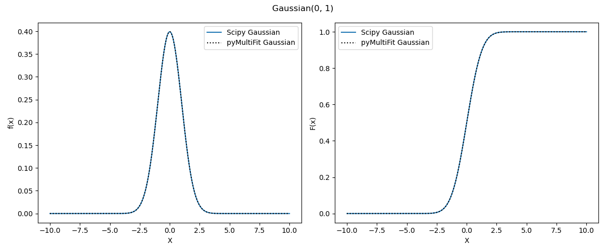
Generating a standard Gaussian(\(\mu=0, \sigma = 1\)) distribution with pyMultiFit and scipy:

x_values = np.linspace(start=-10, stop=10, num=500)

y_multifit = GaussianDistribution(normalize=True)
y_scipy = norm

Plotting PDF and CDF:

f, ax = plt.subplots(1, 2, figsize=(12, 5))

ax[0].plot(x_values, y_scipy.pdf(x=x_values), label='Scipy Gaussian')
ax[0].plot(x_values, y_multifit.pdf(x_values), 'k:', label='pyMultiFit Gaussian')
ax[0].set_ylabel('f(x)')

ax[1].plot(x_values, y_scipy.cdf(x=x_values), label='Scipy Gaussian')
ax[1].plot(x_values, y_multifit.cdf(x_values), 'k:', label='pyMultiFit Gaussian')
ax[1].set_ylabel('F(x)')

f.suptitle('Gaussian(0, 1)')

for i in ax:
    i.set_xlabel('X')
    i.legend()
plt.tight_layout()

Generating a translated Gaussian(\(\mu=3, \sigma=2\)) distribution:

y_multifit = GaussianDistribution(mu=3, std=2, normalize=True)

Plotting PDF and CDF:

f, ax = plt.subplots(1, 2, figsize=(12, 5))

ax[0].plot(x_values, y_scipy.pdf(x=x_values, loc=3, scale=2), label='Scipy translated Gaussian')
ax[0].plot(x_values, y_multifit.pdf(x_values), 'k:', label='pyMultiFit translated Gaussian')
ax[0].set_ylabel('f(x)')

ax[1].plot(x_values, y_scipy.cdf(x=x_values, loc=3, scale=2), label='Scipy translated Gaussian')
ax[1].plot(x_values, y_multifit.cdf(x_values), 'k:', label='pyMultiFit translated Gaussian')
ax[1].set_ylabel('F(x)')

f.suptitle(r'Gaussian(3, 2)')

for i in ax:
    i.set_xlabel('X')
    i.legend()
plt.tight_layout()

cdf(x: ndarray) → ndarray[source]#

Compute the cumulative density function (CDF) for the distribution.

Parameters:: x – Input array at which to evaluate the CDF.

classmethod from_scipy_params(s, loc: float = 0.0, scale: float = 1.0) → LogNormalDistribution[source]#

Instantiate LogNormalDistribution with scipy parametrization.

Parameters:

s: float: The shape parameter.
loc: float, optional: The location parameter. Defaults to 0.0.
scale: float, optional: The scale parameter. Defaults to 1.0.

Returns:

LogNormalDistribution: An instance of normalized LogNormalDistribution.

logcdf(x: ndarray) → ndarray[source]#

Compute the log cumulative density function (logCDF) for the distribution.

Parameters:: x – Input array at which to evaluate the logCDF.

logpdf(x: ndarray) → ndarray[source]#

Compute the log probability density function (logPDF) for the distribution.

Parameters:: x – Input array at which to evaluate the logPDF.

pdf(x: ndarray) → ndarray[source]#

Compute the probability density function (PDF) for the distribution.

Parameters:: x – Input array at which to evaluate the PDF.

classmethod scipy_like(s, loc: float = 0.0, scale: float = 1.0) → LogNormalDistribution[source]#

Instantiate LogNormalDistribution with scipy parametrization.

Parameters:

s: float: The shape parameter.
loc: float, optional: The location parameter. Defaults to 0.0.
scale: float, optional: The scale parameter. Defaults to 1.0.

Returns:

LogNormalDistribution: An instance of normalized LogNormalDistribution.

Deprecated since version 1.0.7: Use from_scipy_params instead of scipy_like. scipy_like will be removed in a future release.

stats() → Dict[str, float][source]#

Computes and returns the statistical properties of the distribution, including,

mean,
median,
variance, and
standard deviation.

Returns:: A dictionary containing statistical properties such as mean, variance, etc.
Return type:: Dict[str, float]

Notes

If any of the parameter is not computable for a distribution, this method returns None.

property mean: float | None#: The mean of the distribution.

property median: float | None#: The median of the distribution.

property mode: float | None#: The mode of the distribution.

property stddev: float | None#: The standard deviation of the distribution.

property variance: float | None#: The variance of the distribution.

This class internally utilizes the following functions from utilities_d module:

Recommended Import#

from pymultifit.distributions import LogNormalDistribution

Full Import#

from pymultifit.distributions.logNormal_d import LogNormalDistribution