Fitting the data: Part 2#
In this tutorial we’ll make use of a data generator with multiple model support, and its respective fitter class.
Quick recap#
Generation of data involves the distributions classes.
In case of multi-modal data, the generators module can be used with
multi_baseormulti_{DISTRIBUTION}function.The fitter module contains pre-defined fitters for \(-\) fitting the data.
Custom data generation#
To generate data using multiple models, e.g., GaussianDistribution + LaplaceDistribution we can make use of the multiple_model function from the generators module.
[1]:
import numpy as np

from pymultifit.generators import multiple_models

fs = 14
Suppose the data follows,
where \(\mathcal{N}\) is the Gaussian and \(\mathcal{L}\) is the Laplace distribution, with their distributions defined as,
and
[2]:
from matplotlib import pyplot as plt
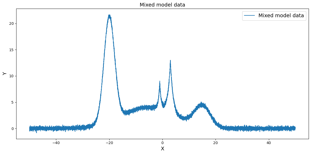
x = np.linspace(-50, 50, 10_000)
parameters = [(20, -20, 2), (4, -5.5, 10), (5, -1, 0.5), (10, 3, 1), (4, 15, 3)]
y_mixed = multiple_models(x, params=parameters,
model_list=['gaussian'] * 2 + ['laplace'] * 2 + ['gaussian'], noise_level=0.2)
plt.figure(figsize=(12, 6))
plt.plot(x, y_mixed, label='Mixed model data')
plt.xlabel('X', fontsize=fs)
plt.ylabel('Y', fontsize=fs)
plt.title('Mixed model data', fontsize=fs)
plt.legend(loc='best', fontsize=fs)
plt.tight_layout()
plt.show()
Let’s break down what’s happening here,
The parameters are defined in a
list of tuple of floatsThe models corresponding to those parameters are given as a list of strings,
['gaussian'] * 2 + ['laplace'] * 2 + ['gaussian']The first set of parameters belong to a gaussian distribution
The second and third set of parameters belong to a laplace distribution
The fourth set of parameters belong to another gaussian distribution
The list of models can also be passed as a single list,
['gaussian', 'gaussian', 'laplace', 'laplace', 'gaussian']and it’ll work the same.
A noise level of 0.2 is passed so that some amount of noise is added to the generated data
Plotting the generated data using
matplotlib
Custom data fitting#
For this kind of data where data is in mixed form, pyMultiFit introduces a powerful class MixedDataFitter. The name implies, it can fit data with mixed distributions, so let’s first import it
[3]:
from pymultifit.fitters import MixedDataFitter
As with all the fitters, it needs,
x_values: The x-values for the data.y_values: The y-values for the data.max_iterations: The max number of iterations for fitting procedure.
But it also requires one additional parameter,
model_list: List of models to fit (e.g.,['gaussian', 'gaussian', 'line']).
Currently, the MixedDataFitter only supports simultaneous fitting of Gaussian, Laplace, LogNormal, SkewNormal, and line function. Work is being done on converting it into a template function as well.
[4]:
mxf = MixedDataFitter(x, y_mixed, ['gaussian', 'gaussian', 'laplace', 'laplace', 'gaussian'])
Taking into consideration that the user might feel ambiguous about calling 'gaussian' vs 'normal' the pyMultiFit has safeguards at string values. One can call, GAUSSIAN, LAPLACE from the pyMultiFit module to remove any responsibility of spell errors,
[5]:
from pymultifit import GAUSSIAN, LAPLACE, NORMAL

mxf2 = MixedDataFitter(x, y_mixed, [GAUSSIAN, NORMAL, LAPLACE, LAPLACE, GAUSSIAN])
With our fitter set, we can now make guesses and try to fit the data
[6]:
amplitudes = [20, 4, 5, 10, 5]
mean = [-20, -6, -1, 2, 10]
std = [2, 8, 0.3, 0.5, 4]

guess = np.column_stack([amplitudes, mean, std])
Now, we pass the guess parameter to our fitter
[7]:
mxf2.fit(p0=guess)
mxf2.plot_fit(show_individuals=True)
[7]:
(<Figure size 1200x600 with 1 Axes>,
 <Axes: title={'center': 'MixedDataFitter fit'}, xlabel='X', ylabel='Y'>)
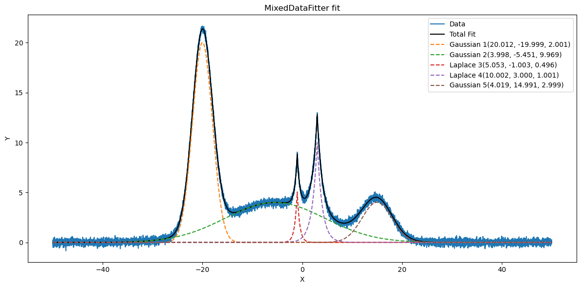
And the data is fitted perfectly, and each fitter’s parameters are also being displayed in the legend.
Exploring the fitted data#
Now that we’ve fitted the data, we want to get the parameters for the fitted values. For this, we can use the handy get_parameters function
[8]:
fitted_parameters = mxf2.get_parameters()
print(fitted_parameters)
{'gaussian': [array([ 20.01160995, -19.99891117, 2.00113134]), array([ 3.99753252, -5.45056598, 9.96936091]), array([ 4.01949018, 14.99111266, 2.99865601])], 'laplace': [array([ 5.05279389, -1.00279685, 0.4956642 ]), array([10.00202108, 2.99976462, 1.00079011])]}
We see here that the get_parameters() function gives the output in form of a dictionary, each model is a key, which has N number of parameters attached to it. In order to get only the values for GAUSSIAN model, we can tell the function to fetch only that.
[9]:
gaussian_values = mxf2.get_parameters(model=GAUSSIAN)
print(gaussian_values)
[array([ 20.01160995, -19.99891117, 2.00113134]), array([ 3.99753252, -5.45056598, 9.96936091]), array([ 4.01949018, 14.99111266, 2.99865601])]
If the errors values are required, we can simply pass True to the get_errors keyword.
[10]:
dict_ = mxf2.get_parameters(model=GAUSSIAN, get_errors=True)

values = dict_['parameters']
errors = dict_['errors']

stacked = np.dstack([values, errors])

for i in range(3):
    print(f'Gaussian {i + 1}\n', stacked[:, i, :])
Gaussian 1
 [[ 2.00116100e+01  1.53659025e-02]
 [-1.99989112e+01  1.52957254e-03]
 [ 2.00113134e+00  1.93577559e-03]]
Gaussian 2
 [[ 3.99753252e+00  7.65244334e-03]
 [-5.45056598e+00  3.82500975e-02]
 [ 9.96936091e+00  3.58446098e-02]]
Gaussian 3
 [[4.01949018e+00 1.27039410e-02]
 [1.49911127e+01 1.08835913e-02]
 [2.99865601e+00 1.25385069e-02]]
Now we have both the parameters, and the errors of the fitted function and their parameters respectively.