Exploring the distributions

So far, we’ve learned how the Distributions work and how to generate them using the BaseDistribution class as well. In this tutorial we’ll explore the distributions some more.

Example 1: \(\mathcal{N}(0, 1)\)

For revision, let’s generate some Gaussian data, \(\mathcal{N}(0, 1)\), using pyMultiFit. For comparison, we will also do the same with scipy.stats.norm.

from scipy.stats import norm

from pymultifit.distributions import GaussianDistribution

fs = 14

The basic generation can be done by calling the class directly as it had default arguments built into it.

multifit_gaussian = GaussianDistribution()
scipy_gaussian = norm()

The GaussianDistribution takes four optional arguments,

• amplitude: The amplitude of the un-normalized Gaussian distribution. Defaults to 1.0.

• mu: The mean of the Gaussian distribution. Defaults to 0.0.

• std: The standard deviation of the Gaussian distribution. Defaults to 1.0.

• normalize: Boolean value to set whether the distribution should be normalized or not. Defaults to False.

For now, we’ll only focus on the mean and standard_deviation parameters, which are by default set to \(0\) and \(1\) respectively. Next, we set up our array and get the Gaussian PDFs to generate the data.

import numpy as np

x = np.linspace(-5, 5, 10_000)

multifit_y = multifit_gaussian.pdf(x)
scipy_y = scipy_gaussian.pdf(x)

Finally, let’s see the plots for both of these distributions,

import matplotlib.pyplot as plt

plt.figure(figsize=(10, 6))

plt.plot(x, multifit_y, ls='-', label=r'pyMultiFit $\mathcal{N}(0, 1)$')
plt.plot(x, scipy_y, ls='--', label=r'scipy $\mathcal{N}(0, 1)$')
plt.xlabel('X', fontsize=fs)
plt.ylabel('Y', fontsize=fs)
plt.title('Gaussian Distribution', fontsize=fs)
plt.tight_layout()
plt.legend(loc='best', fontsize=fs)
plt.show()

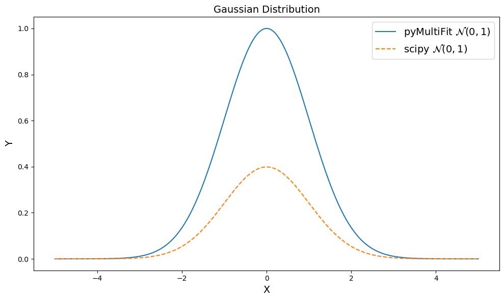
But what’s this? The distributions don’t match.

This is intended, the distribution data created by the pyMultiFit library is intended to be un-normalized, more on this later. In order to generate a normalized distribution, we can set the normalize argument to True.

multifit_gaussian = GaussianDistribution(normalize=True)
multifit_y = multifit_gaussian.pdf(x)

Now, if we re-plot both the distributions, we get,

plt.figure(figsize=(10, 6))

plt.plot(x, multifit_y, ls='-', label='pyMultiFit ' + r'$\mathcal{N}(0, 1)$')
plt.plot(x, scipy_y, ls='--', label='scipy ' + r'$\mathcal{N}(0, 1)$')
plt.xlabel('X', fontsize=fs)
plt.ylabel('Y', fontsize=fs)
plt.title('Gaussian Distribution', fontsize=fs)
plt.legend(loc='best', fontsize=fs)
plt.tight_layout()
plt.show()

Which is exactly what we wanted.

Example 2: \(\mathcal{N}(-2, 0.5)\)

Now let’s see how pyMultiFit handles user defined parameters for GaussianDistribution.

# define N(-2, 0.5) using pyMultiFit and scipy
multifit_gaussian = GaussianDistribution(mu=-2, std=0.5, normalize=True)
scipy_gaussian = norm(loc=-2, scale=0.5)

# generate their PDFs
multifit_y = multifit_gaussian.pdf(x)
scipy_y = scipy_gaussian.pdf(x)

Again, we set normalize keyword to True to get the normalized data. Now, let’s see the two distributions again,

plt.figure(figsize=(10, 6))

plt.plot(x, multifit_y, ls='-', label='pyMultiFit ' + r'$\mathcal{N}(-2, 0.5)$')
plt.plot(x, scipy_y, ls='--', label='scipy ' + r'$\mathcal{N}(-2, 0.5)$')
plt.xlabel('X', fontsize=fs)
plt.ylabel('Y', fontsize=fs)
plt.title('Gaussian Distribution', fontsize=fs)
plt.legend(loc='best', fontsize=fs)
plt.tight_layout()
plt.show()

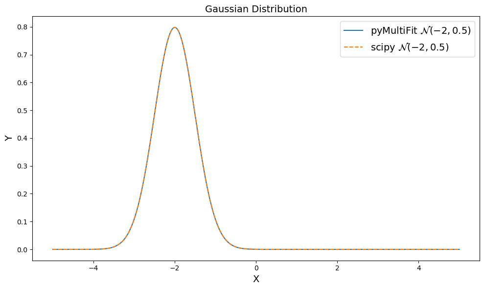
Looks great!

Example 3: \(\mathcal{N}(3, 0.5, 0.5, \text{False})\)

We’ve seen the usage of mean, standard_deviation and normalize parameters, now we’ll learn about the amplitude parameter.

The standard Gaussian distribution is defined as,

\[f(x; \mu, \sigma) = \frac{1}{\sigma\sqrt{2\pi}}\exp\left[-\frac{1}{2}\left(\frac{x - \mu}{\sigma}\right)^2\right]\]

However, this can also be written in terms of amplitude as,

\[f(x; A, \mu, \sigma) = A\exp\left[-\frac{1}{2}\left(\frac{x - \mu}{\sigma}\right)^2\right]\]

where \(A\) now replaces the normalization factor of the distribution as its amplitude. The amplitude parameter forces the distribution to be non-normalized which often reflects the magnitude of the data.

To generate an amplitude-based Gaussian, we can provide the amplitude parameter and keep the normalize parameter as False.

# define amplitude, mean, and standard_deviation for ease of use
amplitude = 3
mean = 0.5
standard_deviation = 0.5

multifit_gaussian = GaussianDistribution(amplitude, mean, standard_deviation)
scipy_gaussian = norm(loc=mean, scale=standard_deviation)

The same can be achieved with scipy as well, but requires some tweakings,

# define the normalization factor to un-normalize scipy distribution
norm_ = np.sqrt(2 * np.pi * standard_deviation**2)

multifit_y = multifit_gaussian.pdf(x)
scipy_y = scipy_gaussian.pdf(x) * (amplitude * norm_)

plt.figure(figsize=(10, 6))

plt.plot(x, multifit_y, ls='-', label='pyMultiFit ' + r'$\mathcal{N}(3, 0.5, 0.5)$')
plt.plot(x, scipy_y, ls='--', label='scipy ' + r'$\mathcal{N}(3, 0.5, 0.5)$')
plt.xlabel('X', fontsize=fs)
plt.ylabel('Y', fontsize=fs)
plt.title('Gaussian Distribution', fontsize=fs)
plt.legend(loc='best', fontsize=fs)
plt.tight_layout()
plt.show()

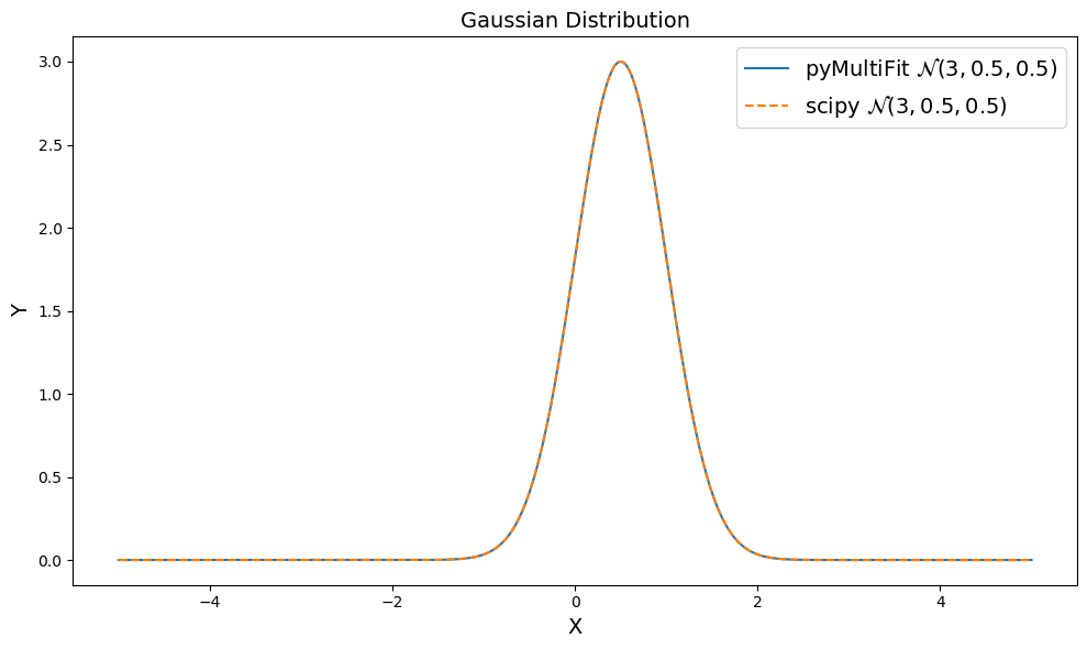
By having a built-in amplitude parameter with normalize parameter, the library allows user to generate both normalized and un-normalized distributions on the go.

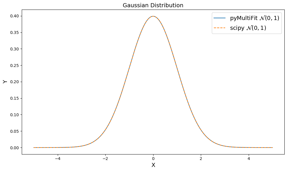
Example 4: \(\mathcal{N}(0, 1)\) using scipy syntax

The scipy library defines the standardized distribution and takes loc and scale as arguments that can provide any type of transformation required by the user. Since most of the people are accustomed to that syntax, and it can take some time to get used to a new syntax, the pyMultiFit library also includes a classmethod for every distribution that encompasses the scipy arguments.

multifit_y = GaussianDistribution.scipy_like().pdf(x)
scipy_y = norm().pdf(x)

The scipy_like takes the exact arguments as the scipy distributions and in the same order to generate scipy_like distributions. Since scipy generates normalized distributions, scipy_like does the same, it generates normalized distributions only.

plt.figure(figsize=(10, 6))

plt.plot(x, multifit_y, ls='-', label='pyMultiFit ' + r'$\mathcal{N}(0, 1)$')
plt.plot(x, scipy_y, ls='--', label='scipy ' + r'$\mathcal{N}(0, 1)$')
plt.xlabel('X', fontsize=fs)
plt.ylabel('Y', fontsize=fs)
plt.title('Gaussian Distribution', fontsize=fs)
plt.legend(loc='best', fontsize=fs)
plt.tight_layout()
plt.show()

This concludes the first exploration tutorial.