Generating N-model data

In the previous tutorial, we constructed the Exponential distribution class using the BaseDistribution class. As a quick recap,

1. The BaseDistribution class has three functions, pdf, cdf, and stats.

2. The API requires a normalize keyword when defining the class.

3. It is better to have PDF and CDF functions separate than the class.

In this tutorial, we’ll focus on the generators module, which helps to generate an N-model distribution over an x array. Just like the BaseDistribution template class, the generators module provides a multi_base function that enables a custom distribution class to be utilized as an N-model generator.

multi_base

The function accepts five arguments,

1. x: The array of values on which the distributions are to be generated,

2. distribution_func: A class/subclass of BaseDistribution,

3. params: List of tuples containing the parameters for the required distribution,

4. noise_level: Standard deviation of the noise to be added to the data, and

5. normalize: Whether to normalize the distribution or not.

Let’s use multi_base to generate the three exponential distributions that we did in the last tutorial with \(\lambda \in [0.5, 1, 1.5]\).

Example 1: Single parameter distribution

Let’s setup our exponential distribution again, but this time using the internal BaseDistribution.

import numpy as np

from pymultifit.distributions.backend import BaseDistribution


def exp_pdf(x, lambda_, normalize: bool = False):
    """Exponential PDF."""
    return lambda_ * np.exp(-lambda_ * x)


def exp_cdf(x, lambda_, normalize: bool = False):
    """Exponential CDF."""
    return 1 - np.exp(-lambda_ * x)


class Exponential(BaseDistribution):
    """Mock Exponential distribution."""

    def __init__(self, lambda_: float = 1.0, normalize: bool = True):
        self.lambda_ = lambda_

        self.norm = normalize

    def pdf(self, x):
        return exp_pdf(x, self.lambda_, self.norm)

    def cdf(self, x):
        return exp_cdf(x, self.lambda_, self.norm)

    def stats(self):
        return {'mean': 1 / self.lambda_}

With the distributions set, we can now generate our three exponentials easily. Let’s define the x-array and distribution parameters. In the case of our exponential distribution, we only need one parameter, \(\lambda\).

Although in this example the parameters are passed as list of floats instead of the intended list of tuples of floats this is because the distribution only requires a single parameter. This will not work with distributions using multiple parameters, as will be demonstrated in the next example.

x_values = np.linspace(0, 10, 5_000)
parameters = [0.5, 1.0, 1.5]

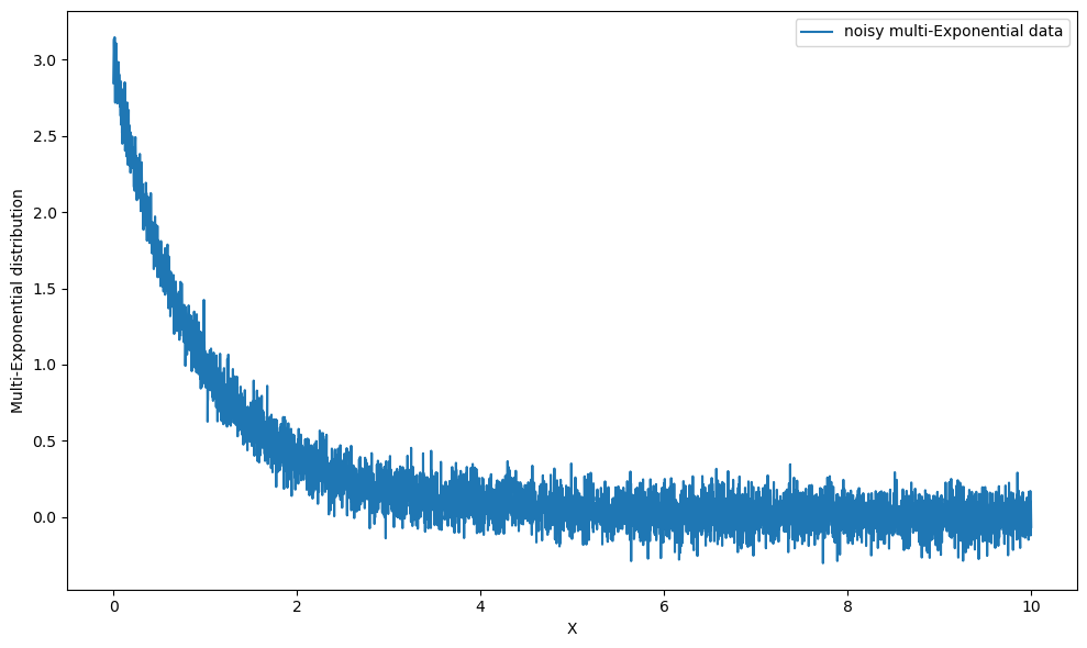
The parameters for the distribution should always be passed as a tuple of parameters, even if it is a single parameter. The normalize parameter is not to be included in the list of parameters here. Let’s also add a small, \(\mathcal{N}(0, 0.1)\) noise to the data.

import matplotlib.pyplot as plt
from pymultifit.generators import multi_base

y_multi_expon = multi_base(x_values,
                           distribution_func=Exponential, params=parameters, noise_level=0.1)

plt.figure(figsize=(10, 6))
plt.plot(x_values, y_multi_expon, label='noisy multi-Exponential data')
plt.xlabel('X')
plt.ylabel('Multi-Exponential distribution')
plt.legend()
plt.tight_layout()
plt.show()

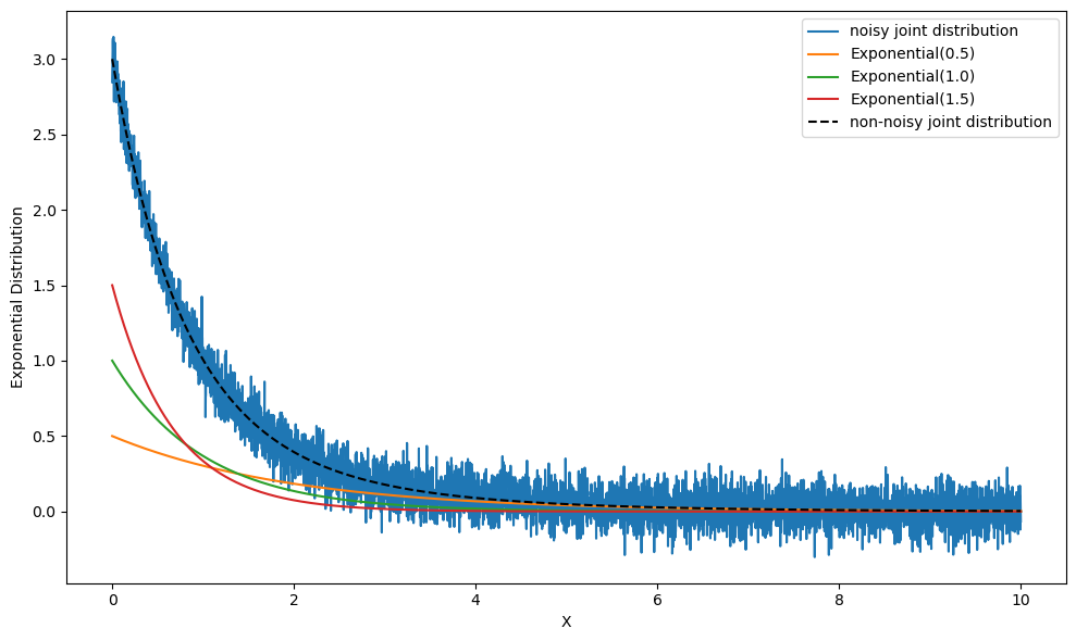
Let’s compare this with our regular three distributions,

exp1 = Exponential(0.5).pdf(x_values)
exp2 = Exponential(1).pdf(x_values)
exp3 = Exponential(1.5).pdf(x_values)

y_expon_sum = exp1 + exp2 + exp3

plt.figure(figsize=(10, 6))
plt.plot(x_values, y_multi_expon, label='noisy joint distribution')
plt.plot(x_values, exp1, label='Exponential(0.5)')
plt.plot(x_values, exp2, label='Exponential(1.0)')
plt.plot(x_values, exp3, label='Exponential(1.5)')
plt.plot(x_values, y_expon_sum, 'k--', label='non-noisy joint distribution')

plt.xlabel('X')
plt.ylabel('Exponential Distribution')
plt.legend()
plt.tight_layout()
plt.show()

Fantastic work!

Example 2: Multi-parameter Distribution

We worked with exponential distribution; now let’s model Gaussian distribution with parameters \(\mu\) and \(\sigma\).

from scipy.special import erf


def gauss_pdf(x,
              mu: float = 0.0, sigma: float = 1.0, normalize: bool = False):
    """Gaussian PDF."""
    exponent = -0.5 * ((x - mu) / sigma)**2
    fraction = np.sqrt(2 * np.pi * sigma**2)

    return np.exp(exponent) / fraction


def gauss_cdf(x,
              mu: float = 0.0, sigma: float = 1.0, normalize: bool = False):
    """Gaussian CDF."""
    num_ = x - mu
    den_ = sigma * np.sqrt(2)
    return 0.5 * (1 + erf(num_ / den_))


class Gaussian(BaseDistribution):
    """Mock Gaussian distribution."""

    def __init__(self,
                 mu: float = 0.0, sigma: float = 1.0,
                 normalize: bool = False):
        self.mu = mu
        self.sigma = sigma
        self.norm = normalize

    def pdf(self, x):
        return gauss_pdf(x, mu=self.mu, sigma=self.sigma, normalize=self.norm)

    def cdf(self, x):
        return gauss_cdf(x, mu=self.mu, sigma=self.sigma, normalize=self.norm)

    def stats(self):
        return {'mean': self.mu}

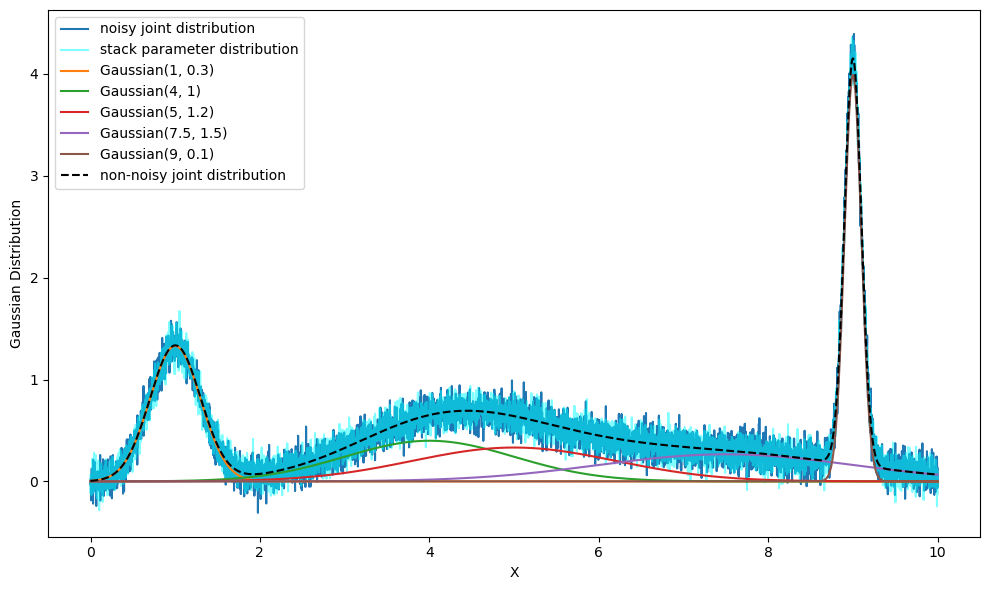
Let’s generate five gaussian distributions with \(\mu \in [1, 4, 5, 7.5, 9]\) and \(\sigma \in [0.3, 1, 1.2, 1.5, 0.1]\) using multi_base.

parameters = [(1, 0.3), (4, 1), (5, 1.2), (7.5, 1.5), (9, 0.1)]

The parameters will always follow the order of the parameters defined in the distribution; in this case, the order of parameters is \((\mu, \sigma)\). Notice the use of tuples here. The parameters are defined in tuples to keep relevant distributions together.

In case you have lists of parameters separately, you can use np.column_stack to reform the lists into a single parsable stack.

mean_list = [1, 4, 5, 7.5, 9]
sigma_list = [0.3, 1, 1.2, 1.5, 0.1]

parameters_stacked = np.column_stack([mean_list, sigma_list])

y_gaussian = multi_base(x_values,
                        distribution_func=Gaussian, params=parameters, noise_level=0.1)

y_gaussian_stacked = multi_base(x_values,
                                distribution_func=Gaussian, params=parameters_stacked, noise_level=0.1)

gaussian_distributions = []

for param in parameters:
    gaussian_distributions.append(Gaussian(mu=param[0], sigma=param[1]).pdf(x_values))

y_gaussian_sum = np.sum(gaussian_distributions, axis=0)

plt.figure(figsize=(10, 6))

# multi-gaussian
plt.plot(x_values, y_gaussian, label='noisy joint distribution')

# multi-gaussian using stacked parameters
plt.plot(x_values, y_gaussian_stacked, 'cyan', alpha=0.5, label='stack parameter distribution')

# individual gaussian distributions
plt.plot(x_values, gaussian_distributions[0], label='Gaussian(1, 0.3)')
plt.plot(x_values, gaussian_distributions[1], label='Gaussian(4, 1)')
plt.plot(x_values, gaussian_distributions[2], label='Gaussian(5, 1.2)')
plt.plot(x_values, gaussian_distributions[3], label='Gaussian(7.5, 1.5)')
plt.plot(x_values, gaussian_distributions[4], label='Gaussian(9, 0.1)')

# summed gaussian distribution
plt.plot(x_values, y_gaussian_sum, 'k--', label='non-noisy joint distribution')

plt.xlabel('X')
plt.ylabel('Gaussian Distribution')
plt.legend()
plt.tight_layout()
plt.show()

And that’s how you generate multi-distribution data using pyMultiFit.