Fitting the data: Part 1

This tutorial will focus on the most important feature of the pyMultiFit library, model fitting.

BaseFitter

Like distributions, the fitters module also provides a handy BaseFitter class for generating a child fitter. The BaseFitter accepts three arguments and one additional class parameter.

1. x_values: The x-values of the data,

2. y_values: The y-values of the data,

3. max_iterations: The maximum number of iterations that the minimizer should follow, and

4. n_par: The number of parameters in the distribution.

It also requires the user to define two methods,

1. fit_boundaries(): It tells the class to keep track of the parameter boundaries.

2. fitter(x, params): The function that can fit the data, e.g., PDF in case of any distribution.

In case the user doesn’t define the boundaries for parameters in the fit_boundaries() function, by default -np.inf and np.inf will be used as lower and upper boundaries, which might not be suitable in all cases. Thus, the user is urged to define the boundaries in the fit_boundaries() function.

The user must provide the fitter function, if not both.

Data generation

Let’s regenerate some normalized multi-Gaussian data with \(\mu = [-20, -5.5, -1, 3, 15]\) and \(\sigma = [2, 5, 0.5, 1, 3]\). For this, we can either define our custom Gaussian class or use the ones provided in the distributions module.

import matplotlib.pyplot as plt
import numpy as np

Let’s create the parameter lists and get them stacked. When using internal GaussianDistribution is it important to note that it uses three parameters instead of two.

1. amplitude: Amplitude, in case of non-normalized distribution generation, \(A\).

2. mean: The mean value, \(\mu\).

3. std: The standard deviation of the Gaussian, \(\sigma\).

For now, since we’re generating normalized Gaussian distributions, and include a nice \(\mathcal{N}(0, 0.01)\) noise in it as well.

For any normalized distribution, the normlize keyword must be set to True whether or not the amplitude is set to 1. This is because the normalize keyword handles the amplitude logic internally.

amplitude = [1, 20, 1, 1, 1]
mu = [-20, -5.5, -1, 3, 15]
sigma = [2, 5, 0.5, 1, 3]

noise_level = 0.01
parameters = np.column_stack([amplitude, mu, sigma])

x_vals = np.linspace(-35, 35, 1500)

The multi-Gaussian data can also be generated by using the multi_gaussian function from the generators module. This removes the need to pass the custom distribution class into the multi_base function.

from pymultifit.generators import multi_gaussian

y_gaussian = multi_gaussian(x_vals, params=parameters, noise_level=noise_level, normalize=True)

plt.figure(figsize=(10, 6))

plt.plot(x_vals, y_gaussian, label='normalized multi-Gaussian')
plt.xlabel('X')
plt.ylabel('Multi-Gaussian')
plt.legend()
plt.tight_layout()
plt.show()

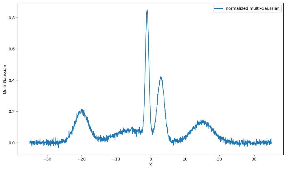
We see here that even though we set the second amplitude parameter to be \(20\), it didn’t scale it because the generator was asked to generate normalized distribution.

Data fitting

Let’s generate a custom fitter using BaseFitter class. The pyMultiFit also provides PDF and CDF functionalities of several distributions via the pymultifit.distributions.utilities_d module.

from pymultifit.fitters.backend import BaseFitter
from pymultifit.distributions.utilities_d import gaussian_pdf_


class CustomFitter(BaseFitter):

    def __init__(self, x_values, y_values, max_iterations: int = 1000):
        super().__init__(x_values=x_values, y_values=y_values, max_iterations=max_iterations)

        # since we're making a Gaussian fitter using pyMultiFit GaussianDistribution,
        # we need three parameters, amplitude, mu, std
        self.n_par = 3

    def fit_boundaries(self):
        lb = (0, -np.inf, 0)
        ub = (np.inf, np.inf, np.inf)

        return lb, ub

    @staticmethod
    def fitter(x, params):
        return gaussian_pdf_(x, *params, normalize=False)

The boundaries are in the same order as those of the input parameters, \(A\), \(\mu\), and \(\sigma\). These are used during the fitting process by scipy.optimize.curve_fit.

Now to fit the data, we pass the x and y values of the data to the custom fitting class we’ve made.

cf = CustomFitter(x_vals, y_gaussian)

Before fitting the data, it can also be visualized via the dry_run method to make some guesses about the parameters.

f, ax = plt.subplots(1, 1, figsize=(10, 6))
cf.dry_run(axis=ax)

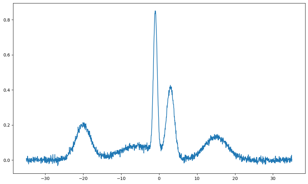
From the plot, we can make some guesses about the parameters

amp_guess = [0.2, 0.1, 0.8, 0.4, 0.1]
mu_guess = [-20, -5, -1, 1, 15]
std_guess = [1, 5, 0.1, 0.1, 0.5]

guesses = np.column_stack([amp_guess, mu_guess, std_guess])

The guesses values are than fed to the fit function of the custom fitter. The fitted data can be visualized via the plot_fit function.

f, ax = plt.subplots(1, 1, figsize=(10, 6))

cf.fit(guesses)
plotter = cf.plot_fit(show_individuals=True, axis=ax)

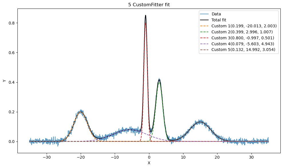
The fitting legends are the result of the show_individual parameter. The labels present the parameters in the same order as the distribution, \(A\), \(\mu\), and \(\sigma\). The amplitude for a normalized distribution is the normalization factor. In case of Gaussian distribution, the amplitude parameter can also be calculated as,

\[A = \dfrac{1}{\sqrt{2\pi\sigma^2}}\]

The output of the plot_fit function is an plt.axes.Axis object that can later be used to apply labels, etcetera if required.