Accuracy#
This benchmark focuses on comparing the accuracy of pyMultiFit’s statistical distributions compared to the well-established SciPy library. The focus is on ensuring that pyMultiFit provides reliable results that closely match theoretical values and SciPy outputs, which are widely trusted in the scientific community.
What is Tested?#
Probability Density Function (PDF): Compares the computed values for given inputs against the expected results and SciPy outputs.
Cumulative Distribution Function (CDF): Verifies that cumulative probabilities match theoretical predictions and SciPy results.
Benchmark setup#
To test accuracy:
Both
pyMultiFitand SciPy are run on the same input data, using distributions like Gaussian, Beta, and Laplace.Results are compared using metrics such as absolute error, relative error, and visual plots.
A range of parameter values and edge cases are included to evaluate robustness and consistency.
Testing#
[1]:
import numpy as np
import scipy.stats as ss

from pymultifit import EPSILON
import pymultifit.distributions as pd
from functions import test_and_plot
[2]:
np.random.seed(43)
[3]:
edge_cases = [np.array([EPSILON, 1e-10, 1e-5, 1, 1e2, 1e3, 1e4, 1e5, 1e7, 0.5e8, 1e10])]
general_cases = [np.logspace(-10, 10, 5_000)]
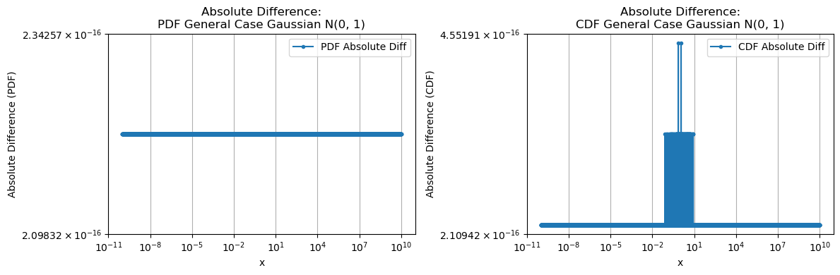
norm(loc=0, scale=1)#
[4]:
custom_dist = pd.GaussianDistribution(normalize=True)
scipy_dist = ss.norm()

test_and_plot(general_case=general_cases, edge_case=edge_cases, custom_dist=custom_dist, scipy_dist=scipy_dist,
              title="Gaussian N(0, 1)")

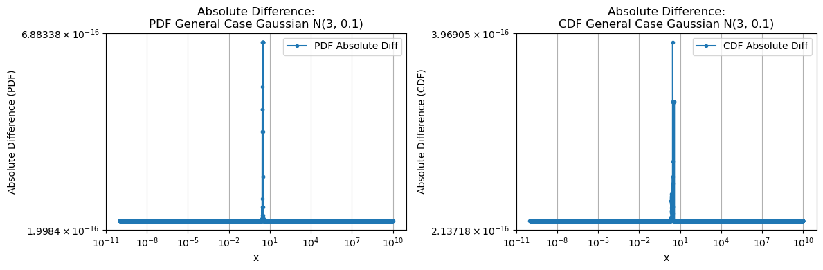
norm(loc=3, scale=0.1)#
[5]:
custom_dist = pd.GaussianDistribution(mean=3, std=0.1, normalize=True)
scipy_dist = ss.norm(loc=3, scale=0.1)

test_and_plot(general_case=general_cases, edge_case=edge_cases, custom_dist=custom_dist, scipy_dist=scipy_dist,
              title='Gaussian N(3, 0.1)')

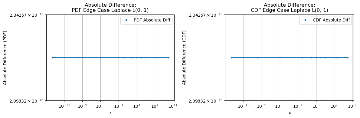
laplace(loc=0, scale=1)#
[6]:
custom_dist = pd.LaplaceDistribution(normalize=True)
scipy_dist = ss.laplace()

test_and_plot(general_case=general_cases, edge_case=edge_cases, custom_dist=custom_dist, scipy_dist=scipy_dist,
              title='Laplace L(0, 1)')

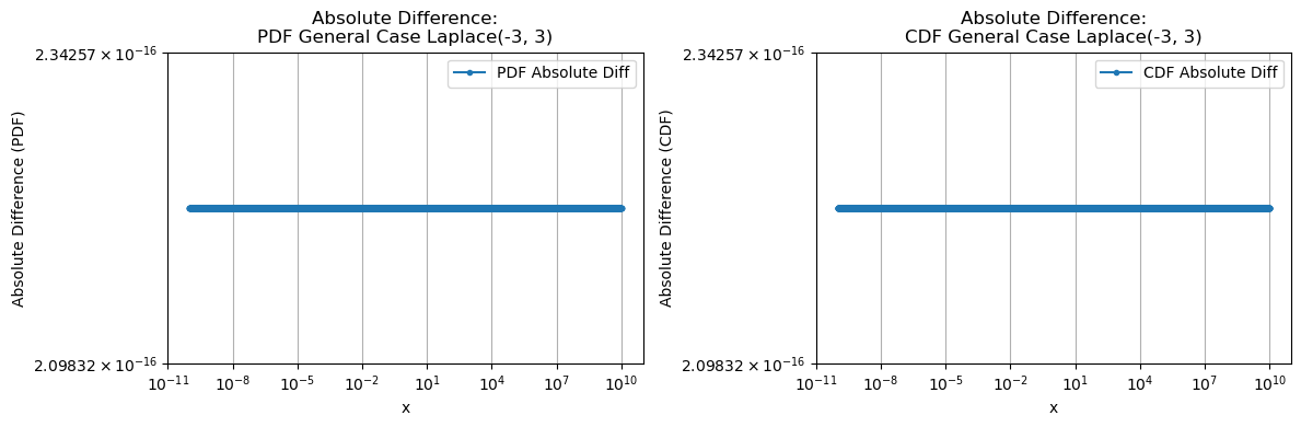
laplace(loc=-3, scale=3)#
[7]:
custom_dist = pd.LaplaceDistribution(mean=-3, diversity=3, normalize=True)
scipy_dist = ss.laplace(loc=-3, scale=3)

test_and_plot(general_case=general_cases, edge_case=edge_cases, custom_dist=custom_dist, scipy_dist=scipy_dist,
              title='Laplace(-3, 3)')

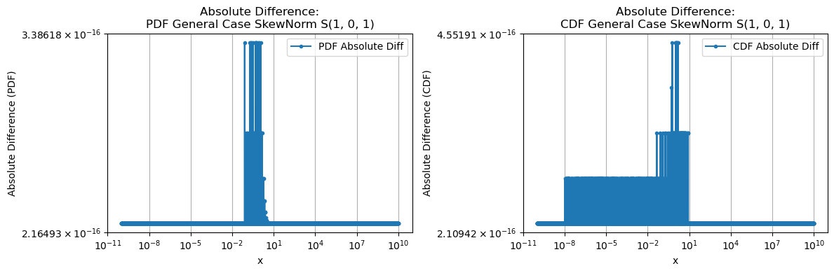
skewnorm(a=1, loc=0, scale=1)#
[8]:
custom_dist = pd.SkewNormalDistribution(normalize=True)
scipy_dist = ss.skewnorm(a=1)

test_and_plot(general_case=general_cases, edge_case=edge_cases, custom_dist=custom_dist, scipy_dist=scipy_dist,
              title='SkewNorm S(1, 0, 1)')

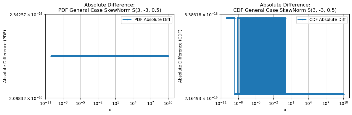
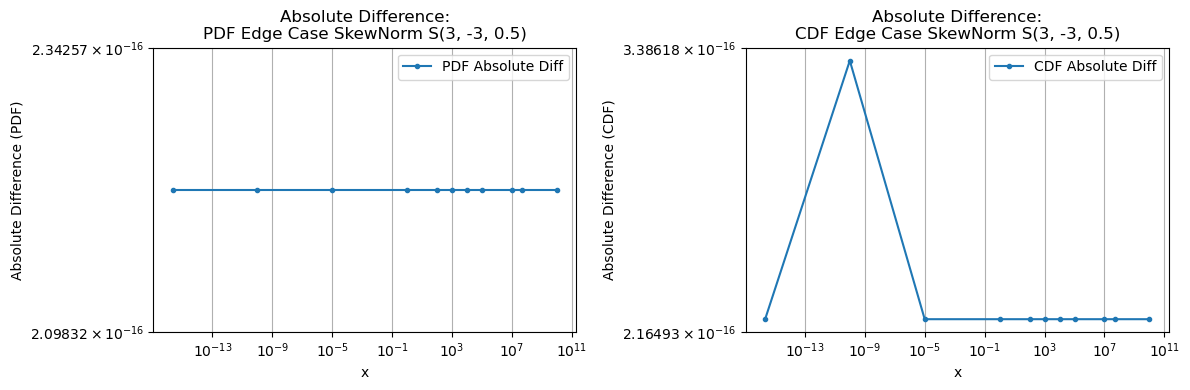
skewnorm(a=3, loc=-3, scale=0.5)#
[9]:
custom_dist = pd.SkewNormalDistribution(shape=3, location=-3, scale=0.5, normalize=True)
scipy_dist = ss.skewnorm(a=3, loc=-3, scale=0.5)

test_and_plot(general_case=general_cases, edge_case=edge_cases, custom_dist=custom_dist, scipy_dist=scipy_dist,
              title='SkewNorm S(3, -3, 0.5)')
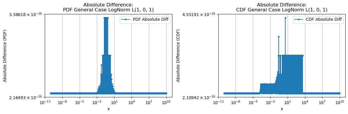
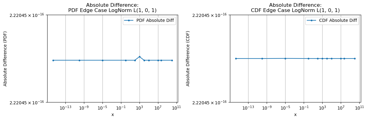
lognorm(s=1, loc=0, scale=1)#
[10]:
custom_dist = pd.LogNormalDistribution(mean=1, std=1, loc=0, normalize=True)
scipy_dist = ss.lognorm(s=1, loc=0, scale=1)

test_and_plot(general_case=general_cases, edge_case=edge_cases, custom_dist=custom_dist, scipy_dist=scipy_dist,
              title='LogNorm L(1, 0, 1)')
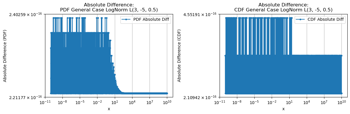
lognorm(s=3, loc=-5, scale=0.5)#
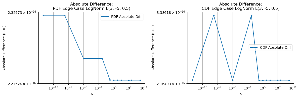
[11]:
custom_dist = pd.LogNormalDistribution(mean=0.5, std=3, loc=-5, normalize=True)
scipy_dist = ss.lognorm(s=3, loc=-5, scale=0.5)

test_and_plot(general_case=general_cases, edge_case=edge_cases, custom_dist=custom_dist, scipy_dist=scipy_dist,
              title='LogNorm L(3, -5, 0.5)')
beta(a=1, b=1)#
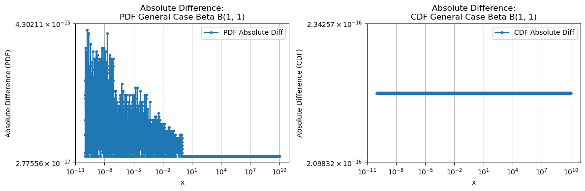
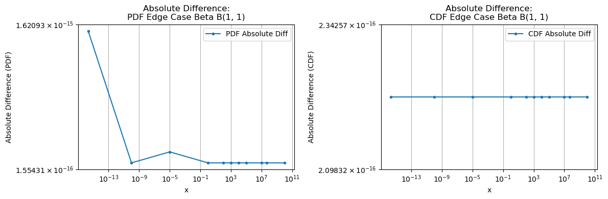
[12]:
custom_dist = pd.BetaDistribution(alpha=1, beta=1, normalize=True)
scipy_dist = ss.beta(a=1, b=1)

test_and_plot(general_case=general_cases, edge_case=edge_cases, custom_dist=custom_dist, scipy_dist=scipy_dist,
              title='Beta B(1, 1)')
beta(a=5, b=80, loc=-3, scale=5)#
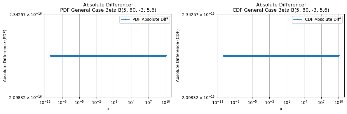
[13]:
custom_dist = pd.BetaDistribution(alpha=5, beta=80, loc=-3, scale=5.6, normalize=True)
scipy_dist = ss.beta(a=5, b=80, loc=-3, scale=5.6)

test_and_plot(general_case=general_cases, edge_case=edge_cases, custom_dist=custom_dist, scipy_dist=scipy_dist,
              title='Beta B(5, 80, -3, 5.6)')
/home/sarl-ws-5/PycharmProjects/pyMultiFit/src/pymultifit/distributions/utilities_d.py:120: RuntimeWarning: overflow encountered in power
  numerator = y**(alpha - 1) * (1 - y)**(beta - 1)
/home/sarl-ws-5/PycharmProjects/pyMultiFit/src/pymultifit/distributions/utilities_d.py:120: RuntimeWarning: overflow encountered in multiply
  numerator = y**(alpha - 1) * (1 - y)**(beta - 1)

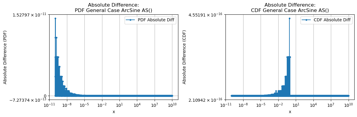
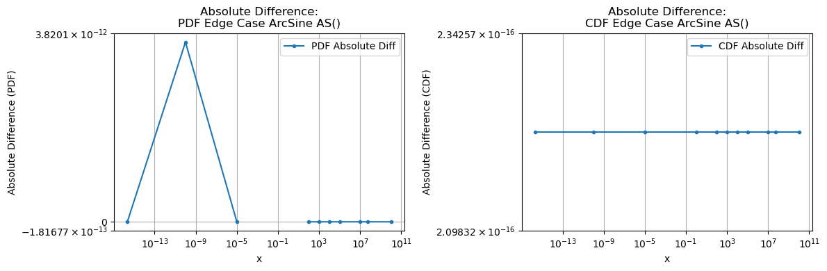
arcsine()#
[14]:
custom_dist = pd.ArcSineDistribution(normalize=True)
scipy_dist = ss.arcsine()

test_and_plot(general_case=general_cases, edge_case=edge_cases, custom_dist=custom_dist, scipy_dist=scipy_dist,
              title='ArcSine AS()')
/home/sarl-ws-5/PycharmProjects/pyMultiFit/src/pymultifit/distributions/utilities_d.py:120: RuntimeWarning: invalid value encountered in power
  numerator = y**(alpha - 1) * (1 - y)**(beta - 1)
/home/sarl-ws-5/PycharmProjects/pyMultiFit/src/pymultifit/distributions/utilities_d.py:120: RuntimeWarning: divide by zero encountered in power
  numerator = y**(alpha - 1) * (1 - y)**(beta - 1)
/home/sarl-ws-5/PycharmProjects/pyMultiFit/benchmarks/functions.py:24: RuntimeWarning: invalid value encountered in subtract
  pdf_abs_diff = np.abs(pdf_custom - pdf_scipy) + EPSILON
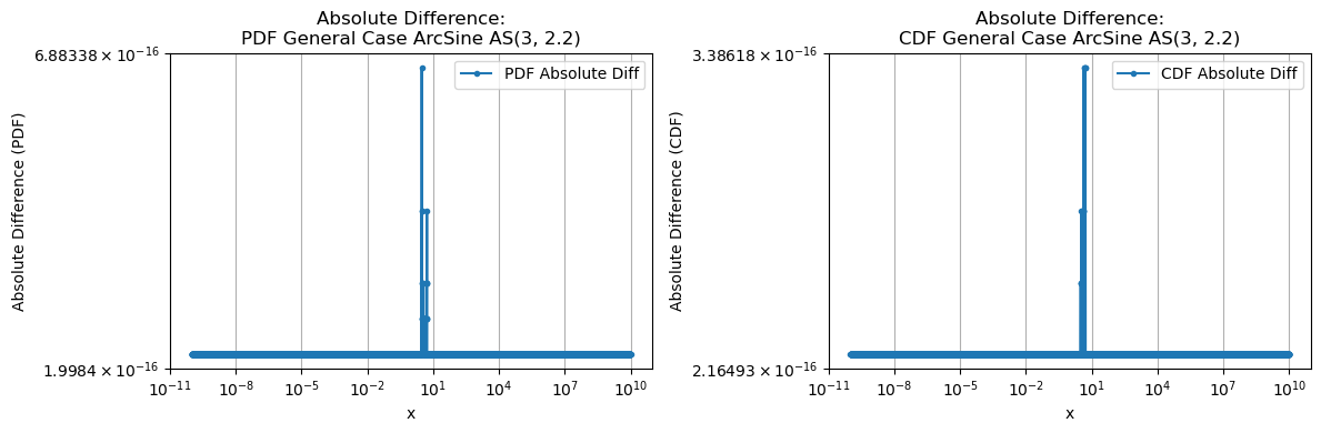
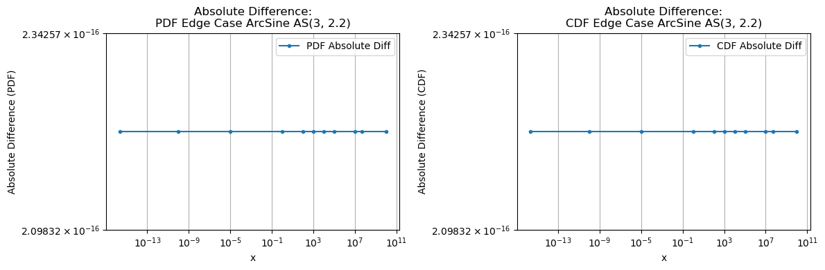
arcsine(loc=3, scale=2.2)#
[15]:
custom_dist = pd.ArcSineDistribution(loc=3, scale=2.2, normalize=True)
scipy_dist = ss.arcsine(loc=3, scale=2.2)

test_and_plot(general_case=general_cases, edge_case=edge_cases, custom_dist=custom_dist, scipy_dist=scipy_dist,
              title='ArcSine AS(3, 2.2)')
gamma(a=1, loc=0, scale=1)#
[16]:
custom_dist = pd.GammaDistributionSS(shape=1, scale=1, loc=0, normalize=True)
scipy_dist = ss.gamma(a=1, loc=0, scale=1)

test_and_plot(general_case=general_cases, edge_case=edge_cases, custom_dist=custom_dist, scipy_dist=scipy_dist,
              title='Gamma G(1, 0, 1)')
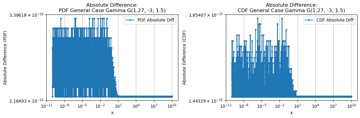
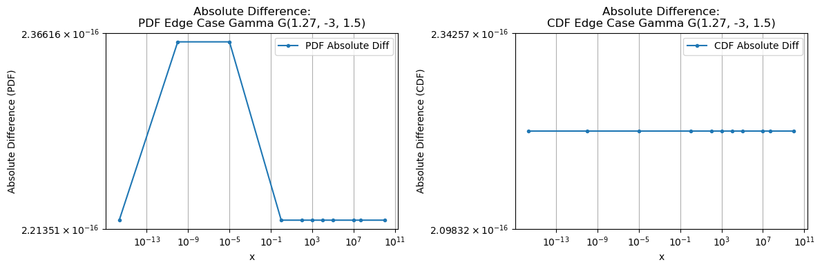
gamma(a=1.27, loc=-3, scale=1.5)#
[17]:
custom_dist = pd.GammaDistributionSS(shape=1.27, scale=1.5, loc=-3, normalize=True)
scipy_dist = ss.gamma(a=1.27, loc=-3, scale=1.5)

test_and_plot(general_case=general_cases, edge_case=edge_cases, custom_dist=custom_dist, scipy_dist=scipy_dist,
              title='Gamma G(1.27, -3, 1.5)')
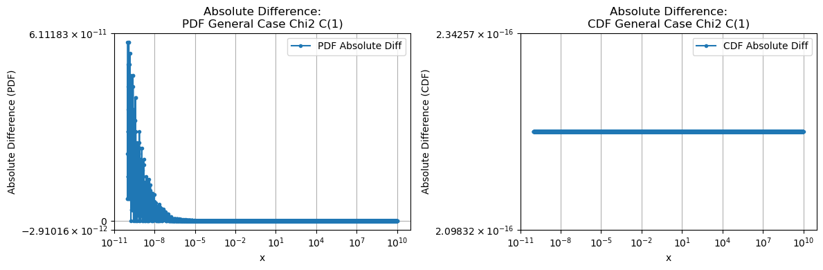
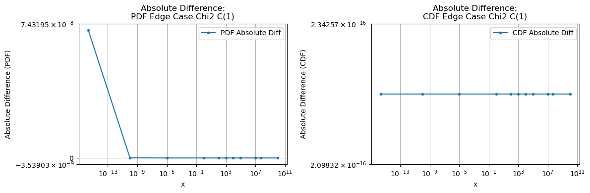
\(\chi^2\)(dof=1)#
[18]:
custom_dist = pd.ChiSquareDistribution(degree_of_freedom=1, normalize=True)
scipy_dist = ss.chi2(df=1)

test_and_plot(general_case=general_cases, edge_case=edge_cases, custom_dist=custom_dist, scipy_dist=scipy_dist,
              title='Chi2 C(1)')
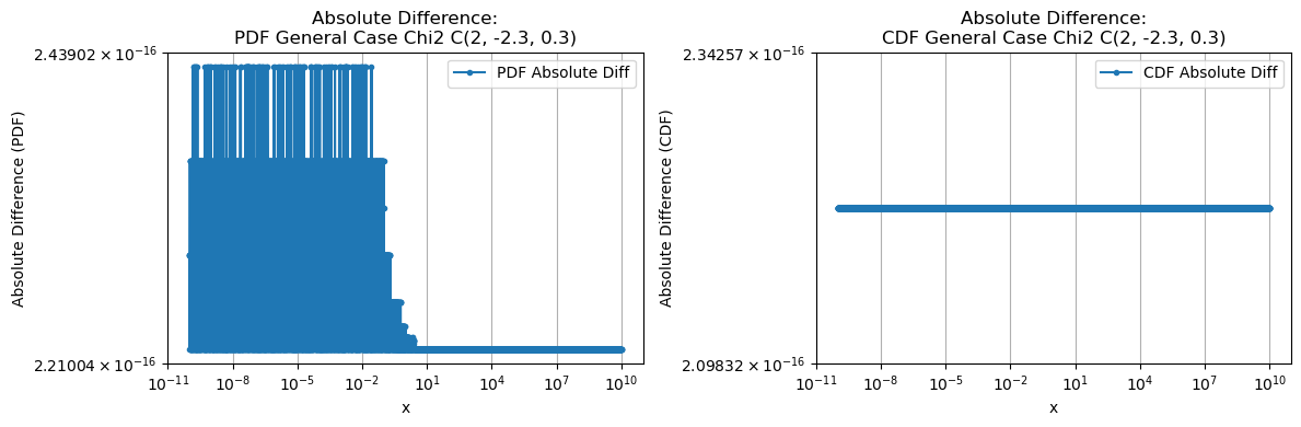
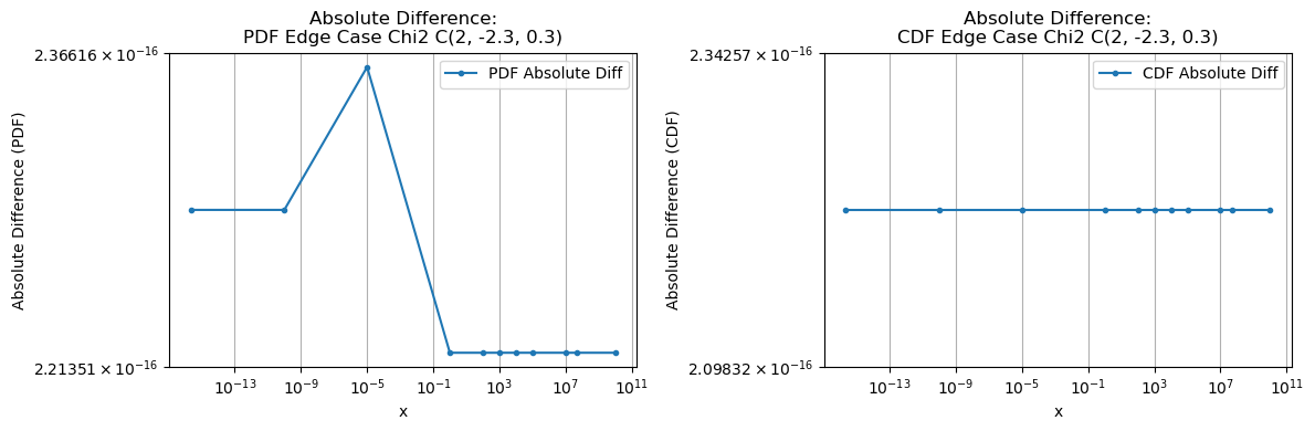
\(\chi^2\)(dof=2, loc=-2.3, scale=0.3)#
[19]:
custom_dist = pd.ChiSquareDistribution(degree_of_freedom=2, loc=-2.3, scale=0.3, normalize=True)
scipy_dist = ss.chi2(df=2, loc=-2.3, scale=0.3)

test_and_plot(general_case=general_cases, edge_case=edge_cases, custom_dist=custom_dist, scipy_dist=scipy_dist,
              title='Chi2 C(2, -2.3, 0.3)')
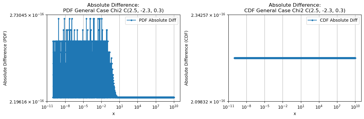
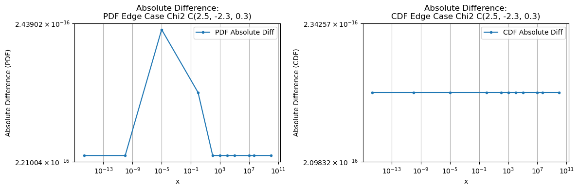
\(\chi^2\)(dof=2.5, loc=-2.3, scale=0.3)#
[20]:
custom_dist = pd.ChiSquareDistribution(degree_of_freedom=2.5, loc=-2.3, scale=0.3, normalize=True)
scipy_dist = ss.chi2(df=2.5, loc=-2.3, scale=0.3)

test_and_plot(general_case=general_cases, edge_case=edge_cases, custom_dist=custom_dist, scipy_dist=scipy_dist,
              title='Chi2 C(2.5, -2.3, 0.3)')
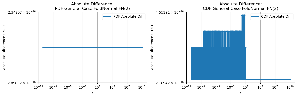
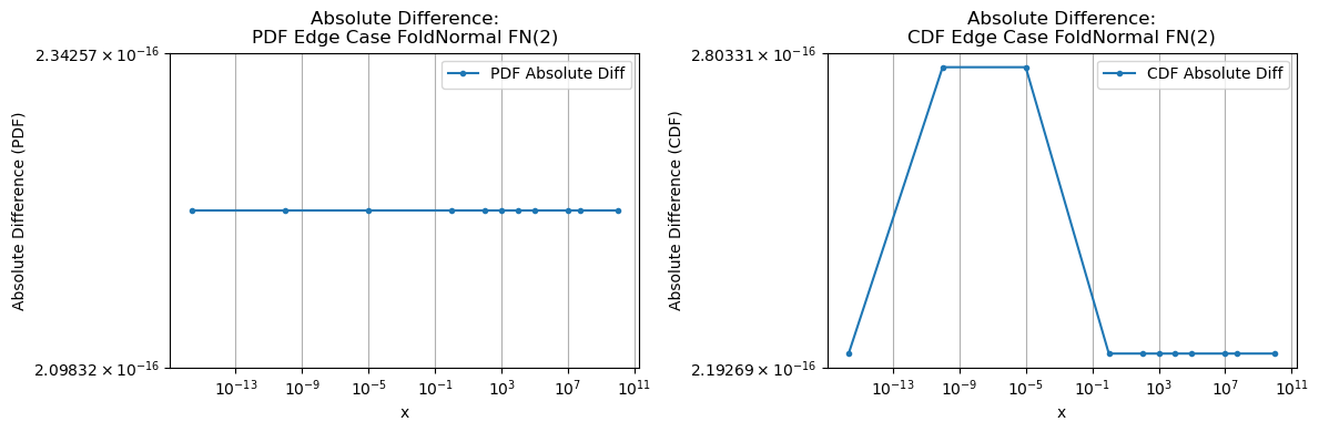
foldnorm(mean=2)#
[21]:
custom_dist = pd.FoldedNormalDistribution(mu=2, normalize=True)
scipy_dist = ss.foldnorm(c=2)

test_and_plot(general_case=general_cases, edge_case=edge_cases, custom_dist=custom_dist, scipy_dist=scipy_dist,
              title='FoldNormal FN(2)')
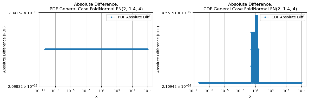
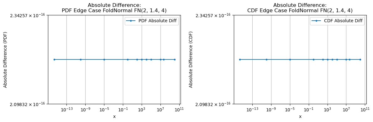
foldnorm(mean=2, loc=1.4, scale=4)#
[22]:
custom_dist = pd.FoldedNormalDistribution(mu=2, sigma=4, loc=1.4, normalize=True)
scipy_dist = ss.foldnorm(c=2, loc=1.4, scale=4)

test_and_plot(general_case=general_cases, edge_case=edge_cases, custom_dist=custom_dist, scipy_dist=scipy_dist,
              title='FoldNormal FN(2, 1.4, 4)')
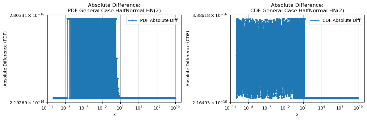
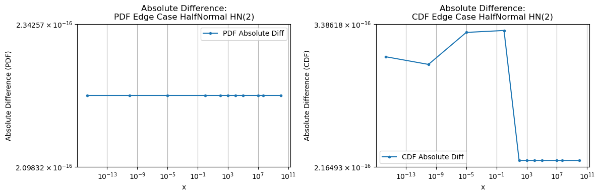
halfNormal(scale=2)#
[23]:
custom_dist = pd.HalfNormalDistribution(scale=2, normalize=True)
scipy_dist = ss.halfnorm(scale=2)

test_and_plot(general_case=general_cases, edge_case=edge_cases, custom_dist=custom_dist, scipy_dist=scipy_dist,
              title='HalfNormal HN(2)')
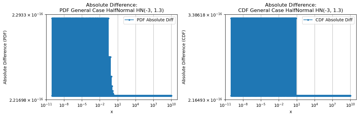
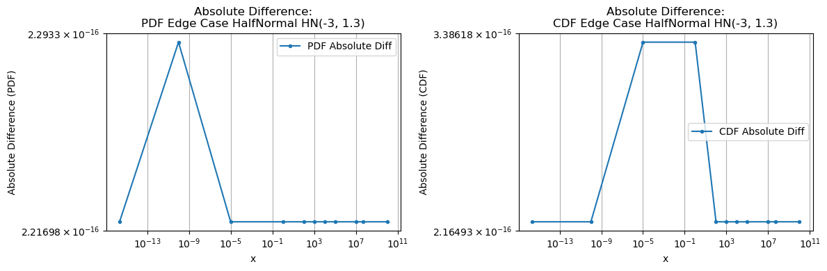
halfnorm(loc=-3, scale=1.3)#
[24]:
custom_dist = pd.HalfNormalDistribution(loc=-3, scale=1.3, normalize=True)
scipy_dist = ss.halfnorm(loc=-3, scale=1.3)

test_and_plot(general_case=general_cases, edge_case=edge_cases, custom_dist=custom_dist, scipy_dist=scipy_dist,
              title='HalfNormal HN(-3, 1.3)')
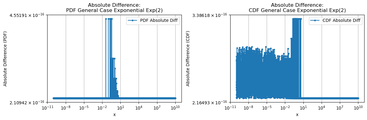
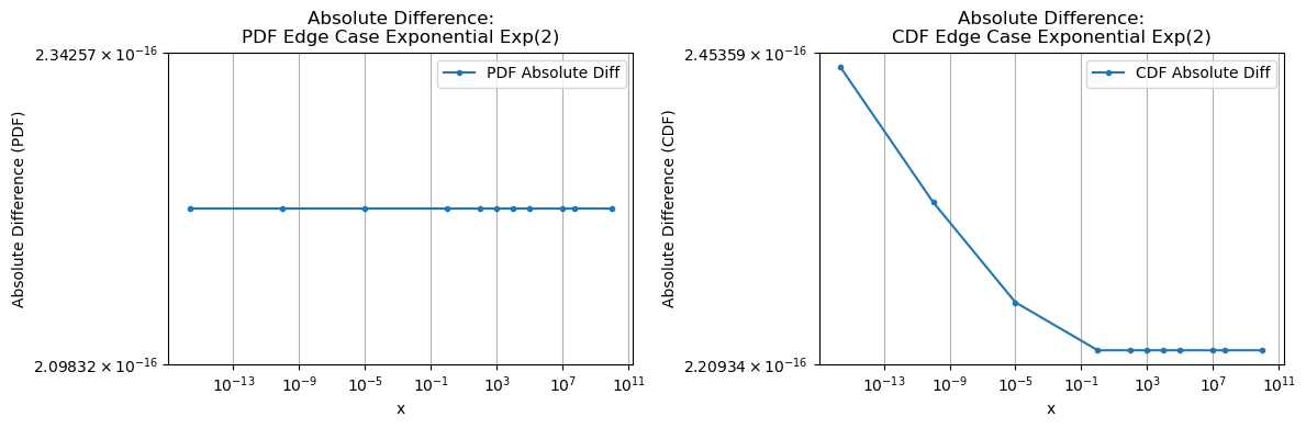
expon(scale=1.4)#
[25]:
custom_dist = pd.ExponentialDistribution(scale=1.4, normalize=True)
scipy_dist = ss.expon(scale=1/1.4)

test_and_plot(general_case=general_cases, edge_case=edge_cases, custom_dist=custom_dist, scipy_dist=scipy_dist,
              title='Exponential Exp(2)')
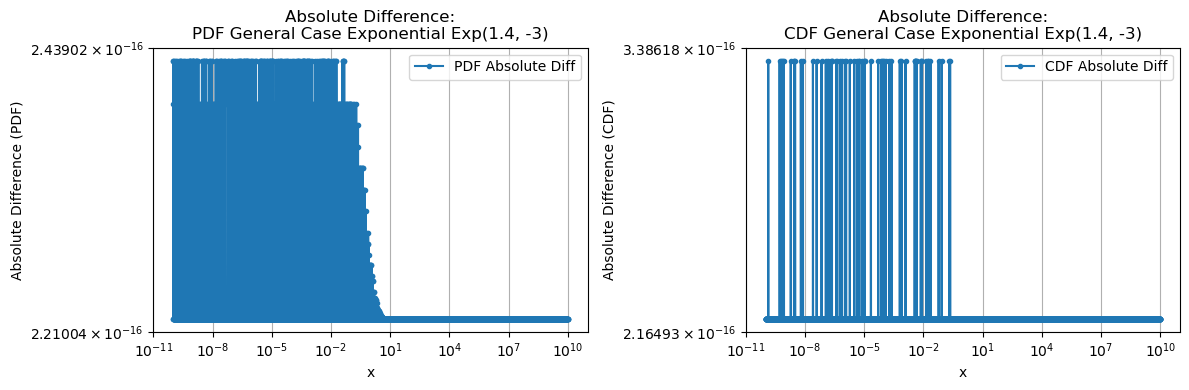
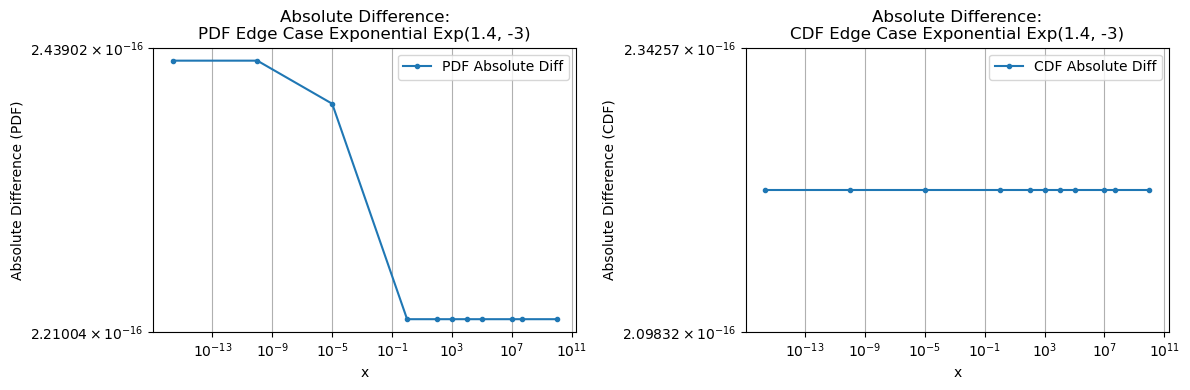
expon(loc=-3, scale=1.4)#
[26]:
custom_dist = pd.ExponentialDistribution(scale=1.4, loc=-3, normalize=True)
scipy_dist = ss.expon(scale=1/1.4, loc=-3)

test_and_plot(general_case=general_cases, edge_case=edge_cases, custom_dist=custom_dist, scipy_dist=scipy_dist,
              title='Exponential Exp(1.4, -3)')