Speed#
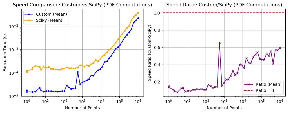
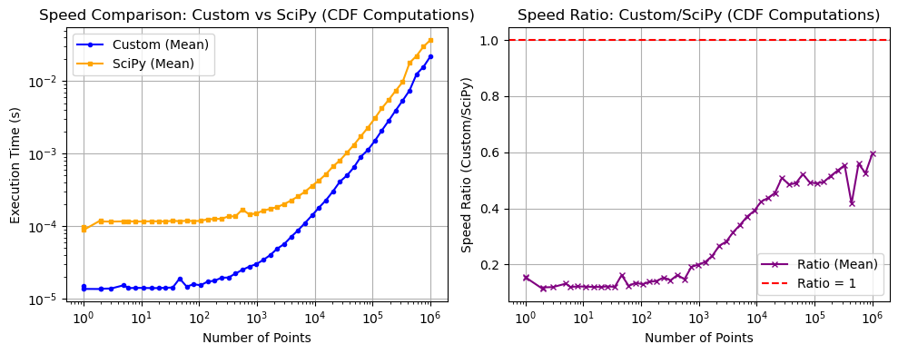
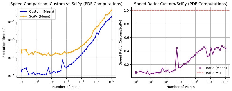
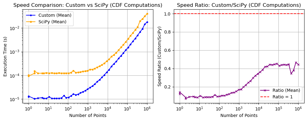
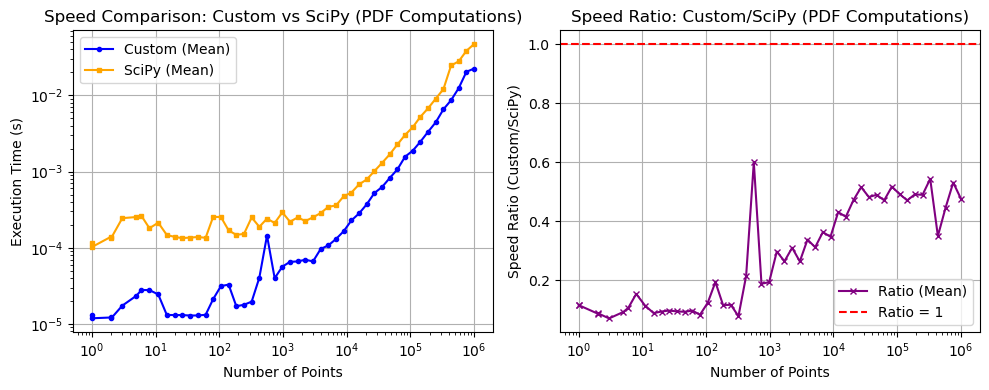
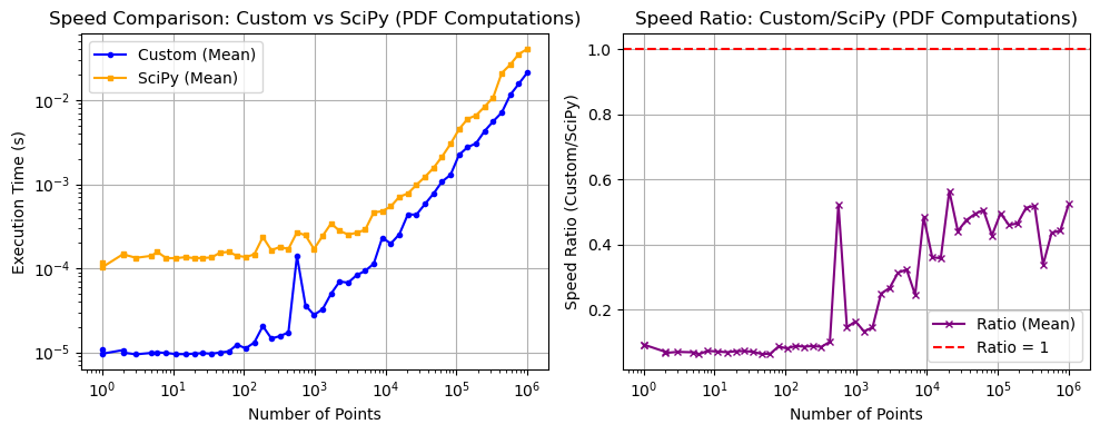
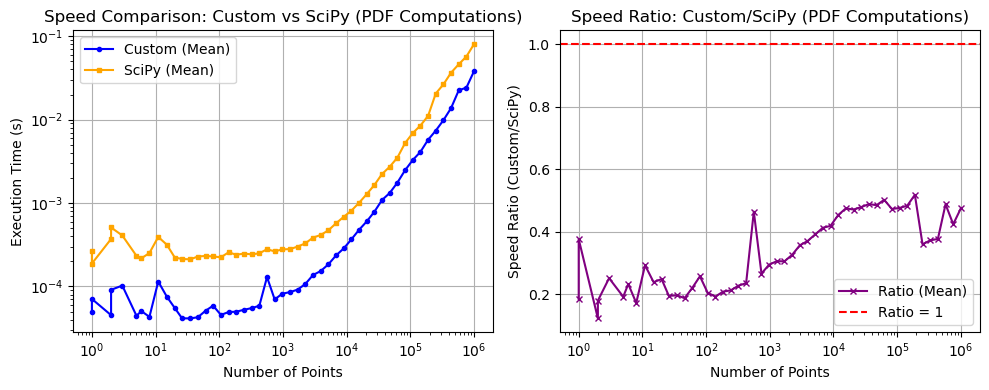
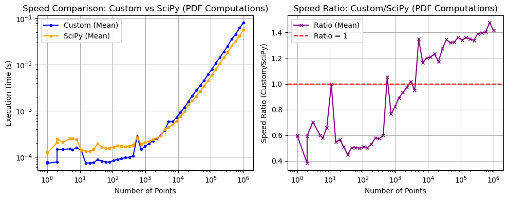
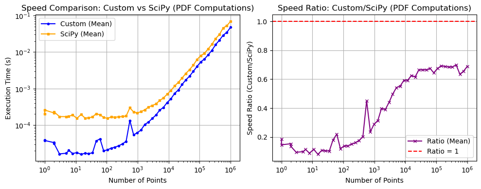
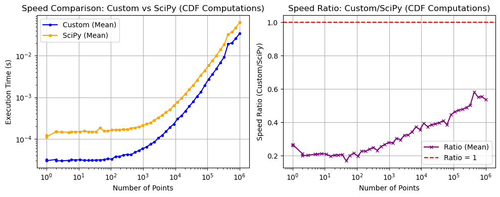
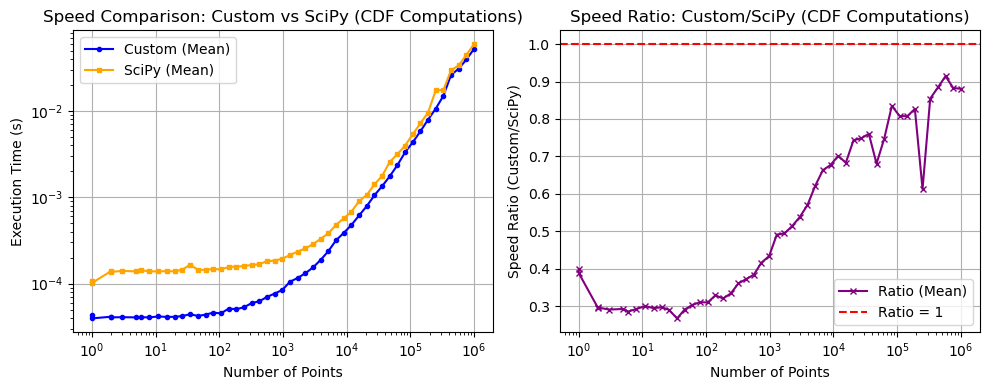
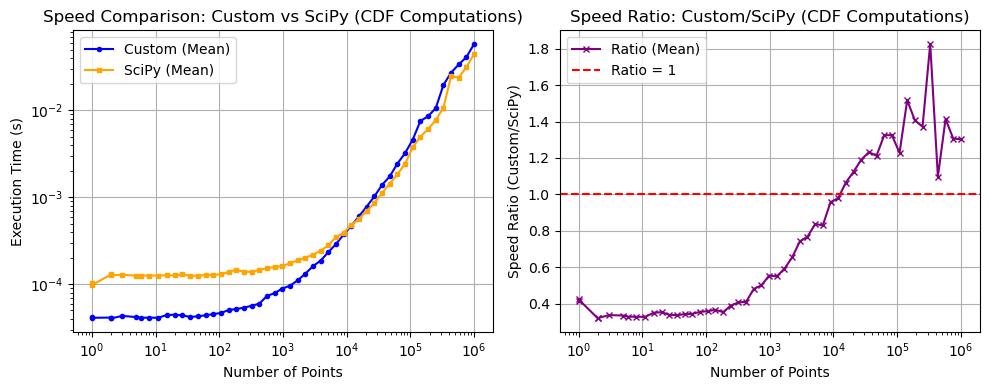
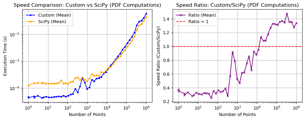
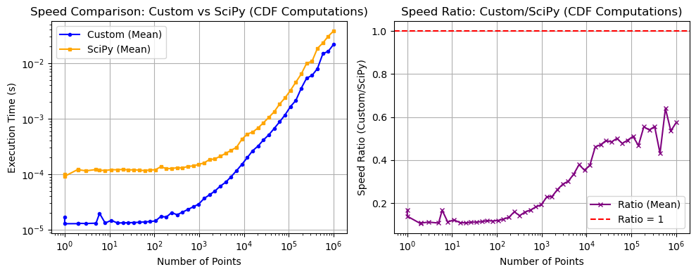
This benchmark focuses on comparing the speed of pyMultiFit’s statistical distribution generations compared to the well-established SciPy library. The focus is on ensuring that pyMultiFit provides reliably faster generation that closely match or are better than SciPy running time.
What is Tested?#
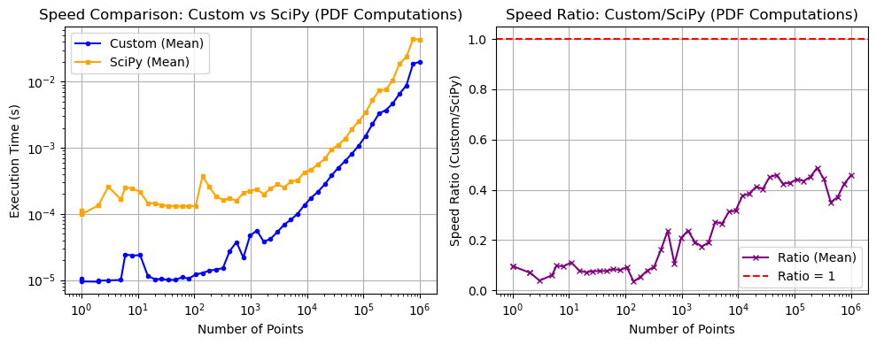
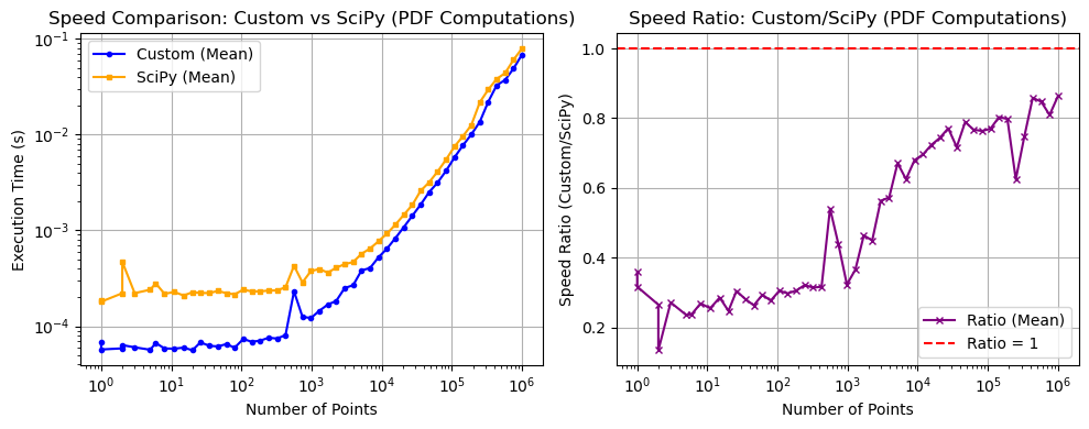
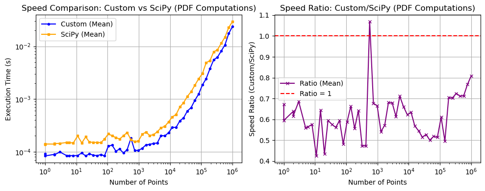
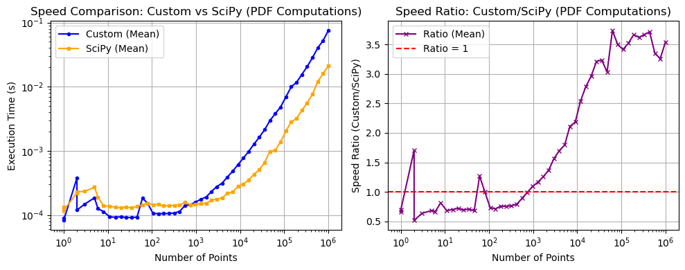
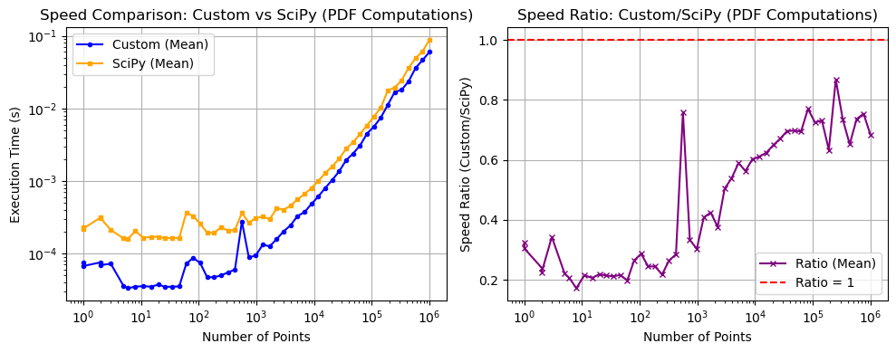
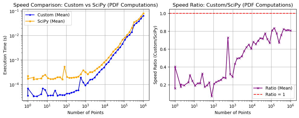
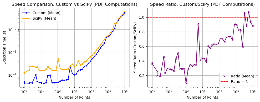
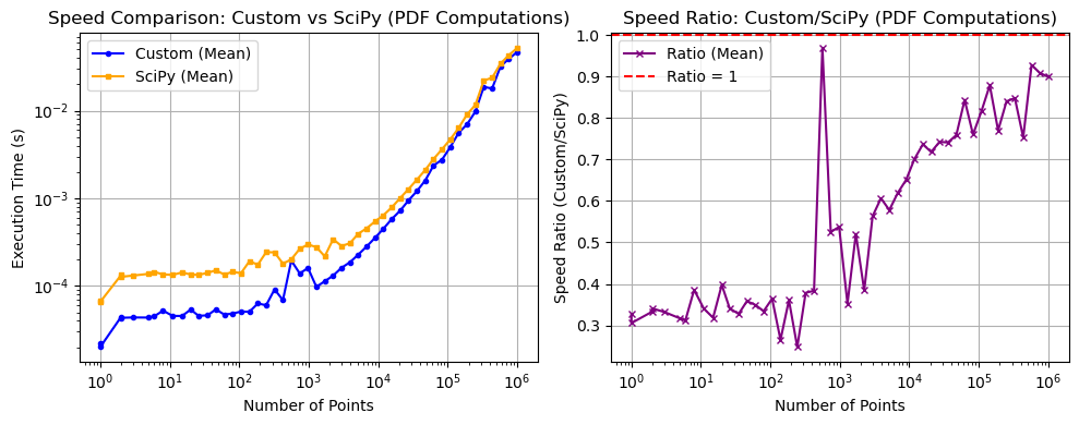
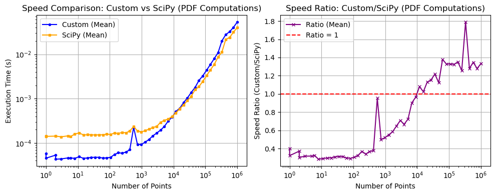
Probability Density Function (PDF): Evaluates the time taken to compute the PDF for a set of input values.
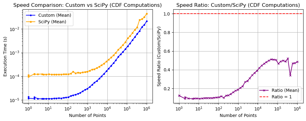
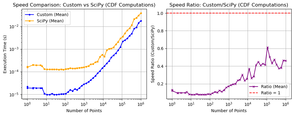
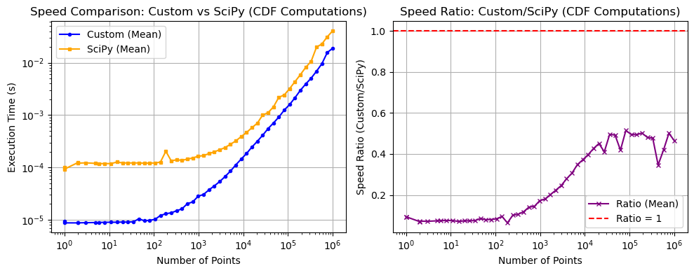
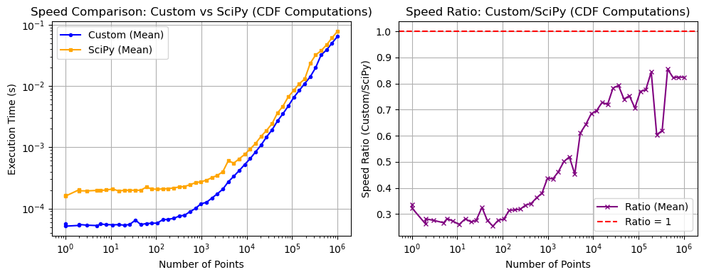
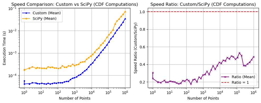
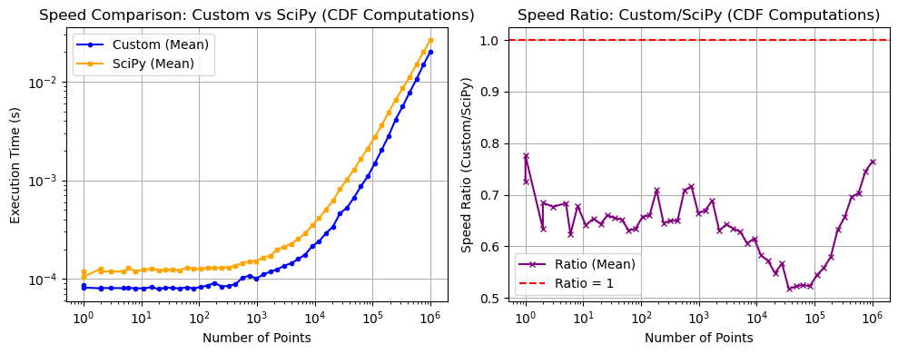
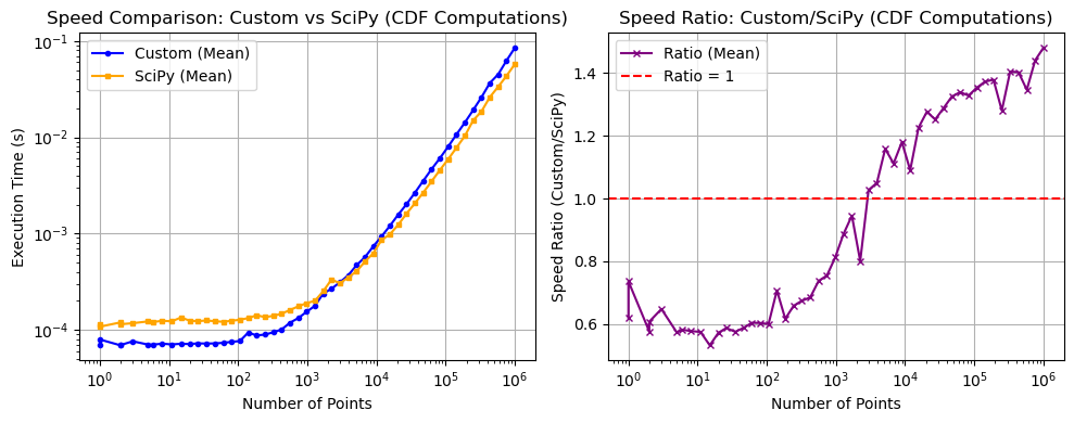
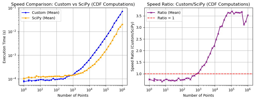
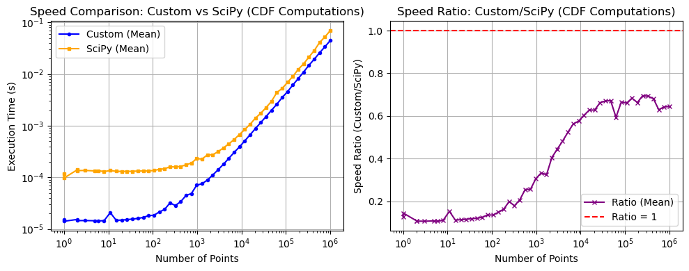
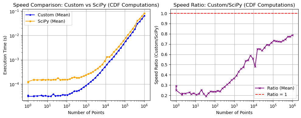
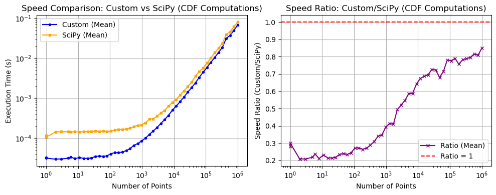
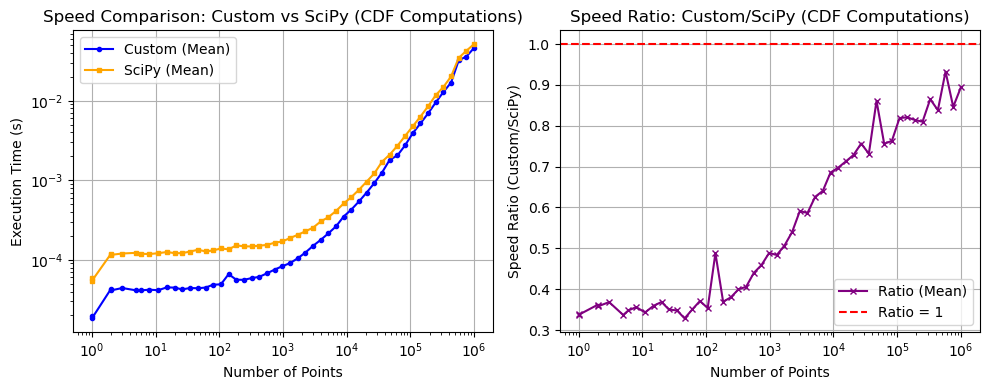
Cumulative Distribution Function (CDF): Measures the performance of computing cumulative probabilities.
Benchmark setup#
To test accuracy:
Both
pyMultiFitand SciPy are run on the same input data, using distributions like Gaussian, Beta, and Laplace.Results are compared using metrics such as absolute error, relative error, and visual plots.
A range of parameter values and edge cases are included to evaluate robustness and consistency.#%% md
Testing#
[1]:
import numpy as np
import scipy.stats as ss

import pymultifit.distributions as pd
from functions import cdf_pdf_plots
[2]:
np.random.seed(43)
n_points_list = np.logspace(0.1, 6, num=50, dtype=int)
normal(loc=0, scale=1)#
[3]:
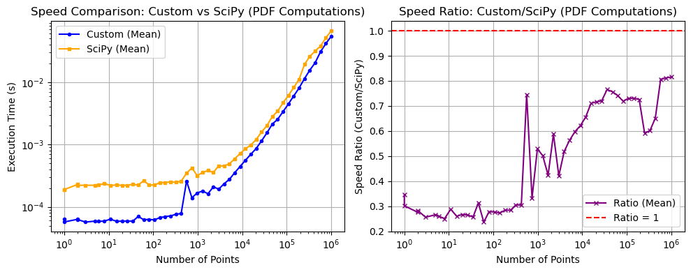
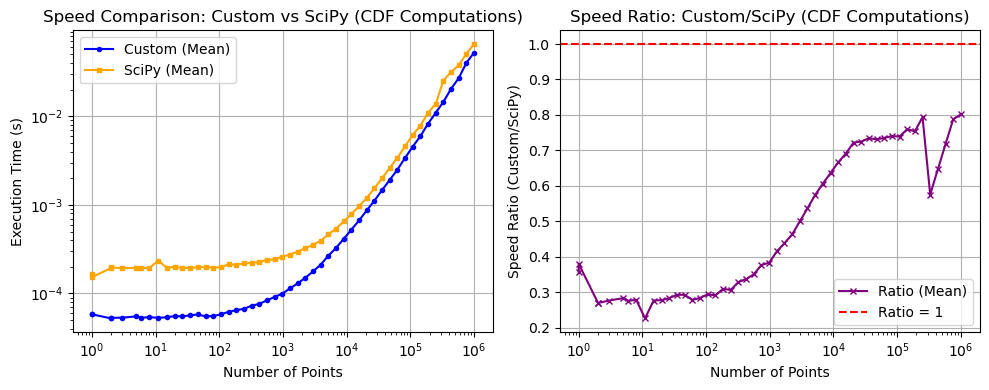
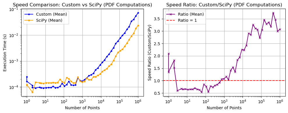
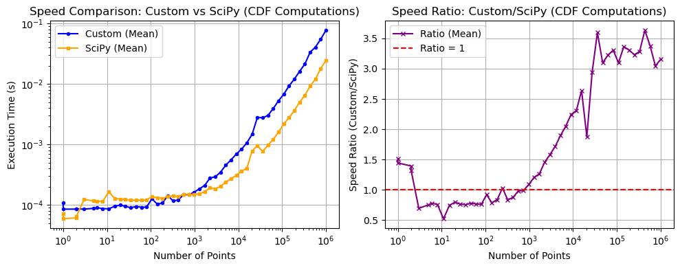
custom_dist = pd.GaussianDistribution(normalize=True)
scipy_dist = ss.norm()

cdf_pdf_plots(custom_dist, scipy_dist, n_points_list, "Gausian N(0, 1)")
normal(loc=3, scale=0.1)#
[4]:
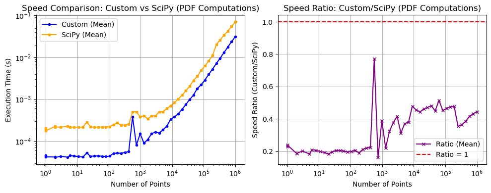
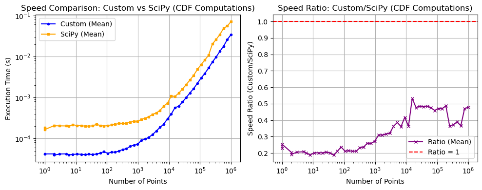
custom_dist = pd.GaussianDistribution(mean=3, std=0.1, normalize=True)
scipy_dist = ss.norm(loc=3, scale=0.1)
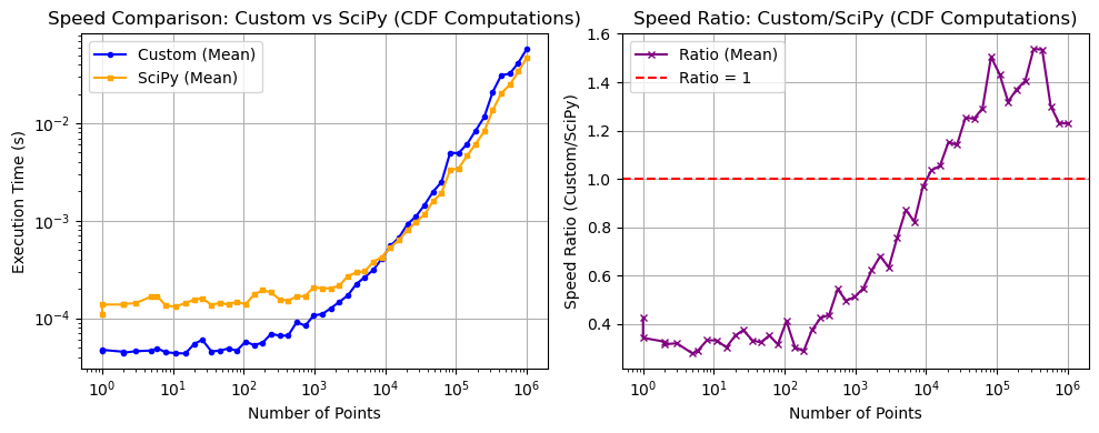
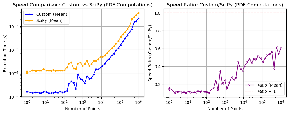
cdf_pdf_plots(custom_dist, scipy_dist, n_points_list, "Gaussian N(3, 0.1)")
laplace(loc=0, scale=1)#
[5]:
custom_dist = pd.LaplaceDistribution(normalize=True)
scipy_dist = ss.laplace()

cdf_pdf_plots(custom_dist, scipy_dist, n_points_list, "Laplace L(0, 1)")
laplace(loc=-3, scale=3)#
[6]:
custom_dist = pd.LaplaceDistribution(mean=-3, diversity=3, normalize=True)
scipy_dist = ss.laplace(loc=-3, scale=3)

cdf_pdf_plots(custom_dist, scipy_dist, n_points_list, "Laplace L(-3, 3)")
skewnorm(a=1, loc=0, scale=1)#
[7]:
custom_dist = pd.SkewNormalDistribution(normalize=True)
scipy_dist = ss.skewnorm(a=1)

cdf_pdf_plots(custom_dist, scipy_dist, n_points_list, "SkewNorm S(1, 0, 1)")
skewnorm(a=3, loc=-3, scale=0.5)#
[8]:
custom_dist = pd.SkewNormalDistribution(shape=3, location=-3, scale=0.5, normalize=True)
scipy_dist = ss.skewnorm(a=3, loc=-3, scale=0.5)

cdf_pdf_plots(custom_dist, scipy_dist, n_points_list, "SkewNorm S(3, -3, 0.5)")
lognorm(s=1, loc=0, scale=1)#
[9]:
custom_dist = pd.LogNormalDistribution(mean=1, std=1, loc=0, normalize=True)
scipy_dist = ss.lognorm(s=1, loc=0, scale=1)

cdf_pdf_plots(custom_dist, scipy_dist, n_points_list, "LogNorm L(1, 0, 1)")
lognorm(s=3, loc=-5, scale=0.5)#
[10]:
custom_dist = pd.LogNormalDistribution(mean=0.5, std=3, loc=-5, normalize=True)
scipy_dist = ss.lognorm(s=3, loc=-5, scale=0.5)

cdf_pdf_plots(custom_dist, scipy_dist, n_points_list, "LogNorm L(3, -5, 0.5)")
beta(a=1, b=1)#
[11]:
custom_dist = pd.BetaDistribution(alpha=1, beta=1, normalize=True)
scipy_dist = ss.beta(a=1, b=1)

cdf_pdf_plots(custom_dist, scipy_dist, n_points_list, "Beta B(1, 1)")
beta(a=5, b=80, loc=-3, scale=5)#
[12]:
custom_dist = pd.BetaDistribution(alpha=5, beta=80, loc=-3, scale=5.6, normalize=True)
scipy_dist = ss.beta(a=5, b=80, loc=-3, scale=5.6)

cdf_pdf_plots(custom_dist, scipy_dist, n_points_list, "Beta B(5, 80, -3, 5.6)")
arcsine()#
[13]:
custom_dist = pd.ArcSineDistribution(normalize=True)
scipy_dist = ss.arcsine()

cdf_pdf_plots(custom_dist, scipy_dist, n_points_list, "ArcSine AS()")
/home/syedalimohsinbukhari/PycharmProjects/pyMultiFit/src/pymultifit/distributions/utilities_d.py:120: RuntimeWarning: invalid value encountered in power
  numerator = y**(alpha - 1) * (1 - y)**(beta - 1)
arcsine(loc=3, scale=2.2)#
[14]:
custom_dist = pd.ArcSineDistribution(loc=3, scale=2.2, normalize=True)
scipy_dist = ss.arcsine(loc=3, scale=2.2)

cdf_pdf_plots(custom_dist, scipy_dist, n_points_list, "AcrSine AS(3, 2.2)")
gamma(a=1, loc=0, scale=1)#
[15]:
custom_dist = pd.GammaDistributionSS(shape=1, scale=1, loc=0, normalize=True)
scipy_dist = ss.gamma(a=1, loc=0, scale=1)

cdf_pdf_plots(custom_dist, scipy_dist, n_points_list, "Gamma G(1, 0, 1)")
gamma(a=1.27, loc=-3, scale=1.5)#
[16]:
custom_dist = pd.GammaDistributionSS(shape=1.27, scale=1.5, loc=-3, normalize=True)
scipy_dist = ss.gamma(a=1.27, loc=-3, scale=1.5)

cdf_pdf_plots(custom_dist, scipy_dist, n_points_list, "Gamma G(1.27, -3, 1.5)")
\(\chi^2\)(dof=1)#
[17]:
custom_dist = pd.ChiSquareDistribution(degree_of_freedom=1, normalize=True)
scipy_dist = ss.chi2(df=1)

cdf_pdf_plots(custom_dist, scipy_dist, n_points_list, "Chi2 C(1)")
\(\chi^2\)(dof=2, loc=-2.3, scale=0.3)#
[18]:
custom_dist = pd.ChiSquareDistribution(degree_of_freedom=2, loc=-2.3, scale=0.3, normalize=True)
scipy_dist = ss.chi2(df=2, loc=-2.3, scale=0.3)

cdf_pdf_plots(custom_dist, scipy_dist, n_points_list, "Chi2 (2, -2.3, 0.3")

\(\chi^2\)(dof=2.5, loc=-2.3, scale=0.3)#
[19]:
custom_dist = pd.ChiSquareDistribution(degree_of_freedom=2.5, loc=-2.3, scale=0.3, normalize=True)
scipy_dist = ss.chi2(df=2.5, loc=-2.3, scale=0.3)

cdf_pdf_plots(custom_dist, scipy_dist, n_points_list, "Chi2 (2.5, -2.3, 0.3")
foldnorm(mean=2)#
[20]:
custom_dist = pd.FoldedNormalDistribution(mean=2, normalize=True)
scipy_dist = ss.foldnorm(c=2)

cdf_pdf_plots(custom_dist, scipy_dist, n_points_list, "FoldNormal FN(2)")
foldnorm(mean=2, loc=1.4, scale=4)#
[21]:
custom_dist = pd.FoldedNormalDistribution(mean=2, sigma=4, loc=1.4, normalize=True)
scipy_dist = ss.foldnorm(c=2, loc=1.4, scale=4)

cdf_pdf_plots(custom_dist, scipy_dist, n_points_list, "FoldNormal FN(2, 1.4, 4)")
halfNormal(scale=2)#
[22]:
custom_dist = pd.HalfNormalDistribution(scale=2, normalize=True)
scipy_dist = ss.halfnorm(scale=2)

cdf_pdf_plots(custom_dist, scipy_dist, n_points_list, "HalfNormal HN(2)")
halfnorm(loc=-3, scale=1.3)#
[23]:
custom_dist = pd.HalfNormalDistribution(loc=-3, scale=1.3, normalize=True)
scipy_dist = ss.halfnorm(loc=-3, scale=1.3)

cdf_pdf_plots(custom_dist, scipy_dist, n_points_list, "HalfNormal HN(-3, 1.3)")
expon(scale=1.4)#
[24]:
custom_dist = pd.ExponentialDistribution(scale=1.4, normalize=True)
scipy_dist = ss.expon(scale=1/1.4)

cdf_pdf_plots(custom_dist, scipy_dist, n_points_list, "Exponential Exp(1.4)")
expon(loc=-3, scale=1.4)#
[25]:
custom_dist = pd.ExponentialDistribution(scale=1.4, loc=-3, normalize=True)
scipy_dist = ss.expon(scale=1/1.4, loc=-3)

cdf_pdf_plots(custom_dist, scipy_dist, n_points_list, "Exponential Exp(-3, 1.4)")